目录：

曲线拟合多项式拟合多项式拟合正弦函数最小二乘拟合Scipy.linalg.lstsq 最小二乘解Scipy.stats.linregress 线性回归更高级的拟合Scipy.optimize.leastsqScipy.optimize.curve_fit

曲线拟合

导入基础包：

import numpy as np
import matplotlib as mpl
import matplotlib.pyplot as plt

plt.rcParams["font.family"] = "SimHei"
plt.rcParams["axes.unicode_minus"] = False

多项式拟合

# 导入线多项式拟合工具：
from numpy import polyfit, poly1d
# 产生数据：
x = np.linspace(-5, 5, 100)
y = 4 * x + 1.5
noise_y = y + np.random.randn(y.shape[-1]) * 2.5

# 画出数据：
%matplotlib inline

p = plt.plot(x, noise_y, 'rx')
p = plt.plot(x, y, 'b:')

进行线性拟合，polyfit
 是多项式拟合函数，线性拟合即一阶多项式：

coeff = polyfit(x, noise_y, 1)
print(coeff)

[3.81313227 1.53189309]

一阶多项式  拟合，返回两个系数 。

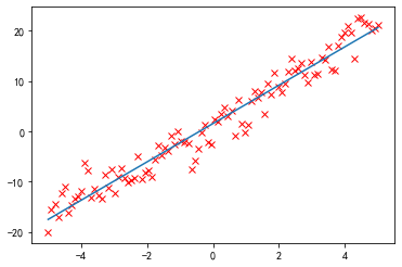
画出拟合曲线：

p = plt.plot(x, noise_y, 'rx')
p = plt.plot(x, y, 'b--')
p = plt.plot(x, coeff[0] * x + coeff[1], 'k-')

还可以用 poly1d
 生成一个以传入的 coeff
 为参数的多项式函数：

f = poly1d(coeff)
p = plt.plot(x, noise_y, 'rx')
p = plt.plot(x, f(x))

display(f)
print(f)

poly1d([3.81313227, 1.53189309])

3.813 x + 1.532

还可以对它进行数学操作生成新的多项式：

print(f + 2 * f ** 2)

       2
29.08 x + 27.18 x + 6.225

多项式拟合正弦函数

正弦函数：

x = np.linspace(-np.pi, np.pi, 100)
y = np.sin(x)

用一阶到九阶多项式拟合，类似泰勒展开：

y1 = poly1d(polyfit(x, y, 1))
y3 = poly1d(polyfit(x, y, 3))
y5 = poly1d(polyfit(x, y, 5))
y7 = poly1d(polyfit(x, y, 7))
y9 = poly1d(polyfit(x, y, 9))

x = np.linspace(-3 * np.pi, 3 * np.pi, 300)

p = plt.plot(x, np.sin(x), 'k', label="sin(x)")
p = plt.plot(x, y1(x), label="1")
p = plt.plot(x, y3(x), label="3")
p = plt.plot(x, y5(x), label="5")
p = plt.plot(x, y7(x), label="7")
p = plt.plot(x, y9(x), label="9")

a = plt.axis([-3 * np.pi, 3 * np.pi, -1.25, 1.25])
plt.legend()
plt.show()

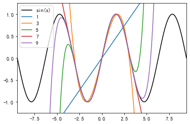
黑色为原始的图形，可以看到，随着多项式拟合的阶数的增加，曲线与拟合数据的吻合程度在逐渐增大。

最小二乘拟合

导入相关的模块：

from scipy.linalg import lstsq
from scipy.stats import linregress

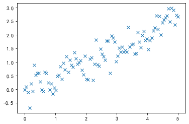
x = np.linspace(0, 5, 100)
y = 0.5 * x + np.random.randn(x.shape[-1]) * 0.35

plt.plot(x, y, 'x')

[<matplotlib.lines.Line2D at 0x1757efd0>]

Scipy.linalg.lstsq 最小二乘解

一般，当使用一个 N-1 阶的多项式拟合这 M 个点时，有这样的关系存在：

即

要得到 C
 ，可以使用 scipy.linalg.lstsq
 求最小二乘解。

这里，我们使用 1 阶多项式即 N = 2
，先将 x
 扩展成 X
：

x = np.linspace(0, 5, 100)
h = np.random.randn(x.shape[-1]) * 0.8
y = 0.7 * x + h
print(f"原函数f(x)=0.7x+0.8*N(0,1)")
X = np.hstack((x[:, np.newaxis], np.ones((x.shape[-1], 1))))
# 求解：
C, resid, rank, s = lstsq(X, y)
print(f"拟合函数f(x)={C[0]}x+{C[1]}")
print(f"残差平方和(sum squared residual) = {resid:.3f}")
print(f"矩阵X的秩(rank of the X matrix) = {rank}")
print(f"奇异值分解(singular values of X) = {s}")
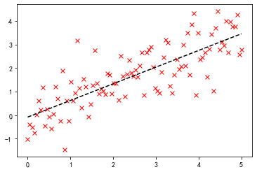
# 画图：
p = plt.plot(x, y, 'rx')
p = plt.plot(x, C[0] * x + C[1], 'k--')

原函数f(x)=0.7x+0.8*N(0,1)
拟合函数f(x)=0.7074763635934755x+-0.08249211243588586
残差平方和(sum squared residual) = 63.276
矩阵X的秩(rank of the X matrix) = 2
奇异值分解(singular values of X) = [30.23732043  4.82146667]

Scipy.stats.linregress 线性回归

slope, intercept, r_value, p_value, stderr = linregress(x, y)
print("原函数f(x)=0.7x+0.8*N(0,1)")
print(f"拟合函数f(x)={slope}x+{intercept}")
print(f"R-value = {r_value:.3f}")
print(f"p-value (probability there is no correlation) = {p_value:.3e}")
print(f"均方误差RMSE(Root mean squared error of the fit) = {np.sqrt(stderr):.3f}")

p = plt.plot(x, y, 'rx')
p = plt.plot(x, slope * x + intercept, 'k--')

原函数f(x)=0.7x+0.8*N(0,1)
拟合函数f(x)=0.7074763635934755x+-0.08249211243588661
R-value = 0.792
p-value (probability there is no correlation) = 1.036e-22
均方误差RMSE(Root mean squared error of the fit) = 0.235

可以看到，两者求解的结果是一致的，但是出发的角度是不同的。

更高级的拟合

定义非线性函数：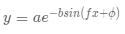

def function(x, a , b, f, phi):
    result = a * np.exp(-b * np.sin(f * x + phi))
    return result

from scipy.optimize import leastsq

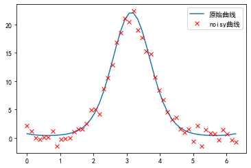
x = np.linspace(0, 2 * np.pi, 50)
actual_parameters = [3, 2, 1.25, np.pi / 4]
y = function(x, *actual_parameters)
# 画出原始曲线：
p = plt.plot(x, y, label="原始曲线")

# 加入噪声：
from scipy.stats import norm
y_noisy = y + 0.9 * norm.rvs(size=len(x))
p = plt.plot(x, y_noisy, 'rx', label="noisy曲线")

plt.legend()

<matplotlib.legend.Legend at 0xfea9ef0>

Scipy.optimize.leastsq

定义误差函数，将要优化的参数放在前面：

def f_err(p, y, x):
    return y - function(x, *p)

将这个函数作为参数传入 leastsq
 函数，第二个参数为初始值：

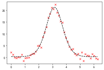
c, ret_val = leastsq(f_err, [1, 1, 1, 1], args=(y_noisy, x))
c, ret_val

(array([2.45649947, 2.16216292, 1.1618549 , 1.06139211]), 1)

ret_val
 是 1~4 时，表示成功找到最小二乘解：

p = plt.plot(x, y_noisy, 'rx')
p = plt.plot(x, function(x, *c), 'k--')

Scipy.optimize.curve_fit

更高级的做法：

from scipy.optimize import curve_fit
# 不需要定义误差函数，直接传入 function 作为参数：
p_est, err_est = curve_fit(function, x, y_noisy)
# 函数的参数
print("函数的参数:", p_est)
print("协方差矩阵:\n", err_est)
p = plt.plot(x, y_noisy, "rx")
p = plt.plot(x, function(x, *p_est), "k--")

函数的参数: [2.45649949 2.16216291 1.1618549  1.0613921 ]
协方差矩阵:
 [[ 0.56326029 -0.22664715  0.07116718 -0.22363429]
 [-0.22664715  0.0915539  -0.02843914  0.08936659]
 [ 0.07116718 -0.02843914  0.00955867 -0.03003698]
 [-0.22363429  0.08936659 -0.03003698  0.09462869]]

协方差矩阵的对角线为各个参数的方差：

print("协方差矩阵的对角线为各个参数的方差(normalized relative errors for each parameter)：")
print("   a\t  b\t f\tphi")
print(np.sqrt(err_est.diagonal()) / p_est)

协方差矩阵的对角线为各个参数的方差(normalized relative errors for each parameter)：
   a      b  f  phi
[0.30551876 0.13994263 0.0841486  0.28982481]