GraphSAGE论文总结

本次要总结的是 论文 Inductive Representation Learning on Large Graphs^[1]，参考的实现代码链接code^[2]，本篇论文是GNN领域内一篇非常重要的论文，值得认真读下。

「建议在非深色主题下阅读本文，pc端阅读点击文末左下角“阅读原文”，体验更佳」

文章目录

• 论文动机和创新点

• 之前相关工作

• 基于matrix-factorization的一些方法（Graph Embedding方法）

• Graph convolutional networks方法

• 模型

• Embedding generation algorithm

• 邻居节点的定义

• GraphSAGE模型的参数学习

• 聚合函数选择

• GraphSAGE(Mean aggregator) 与 GCN比较

• 实验

• 分类实验效果如下：

• 运行效率对比

• 核心代码分析

• 数据预处理

• MeanAggregator

• encoder

• 模型训练和预测

• 个人总结

论文动机和创新点

• 将大图中的节点用低维度的稠密向量表示，已经被证明是非常有用的方法，但是现有的大部分方法，都是将图中的所有节点扔进模型中进行训练，本质还是直推式的，其训练得到的模型不容易推广到未见过的节点，或者一张新的图上。本论文涉及两个重要概念，分别如下：transductive：直推式，不能推广到未见过的节点；inductive：归纳式，能很容易的推广到未见过的节点，适用于变化的图

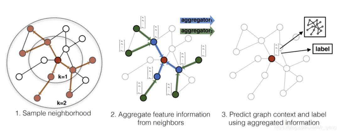
• 本论文提出了GraphSAGE模型，是一种在图上的通用的归纳式的框架，利用节点特征信息（例如文本属性）来高效地为训练阶段未见节点生成embedding。该模型学习的不是节点的embedding向量，而是学习一种聚合方式，即如何通过从一个节点的局部邻居采样并聚合顶点特征，得到节点最终embedding表征。当学习到适合的聚合函数后，可以迅速应用到未见过的图上，得到未见过的节点embedding。

• 本论文提出GraphSAGE模型，既可以用无监督的方式得到节点embedding，供下游任务使用，也可以进行端到端的训练，例如节点分类任务。

之前相关工作

基于matrix-factorization的一些方法（Graph Embedding方法）

• Grarep: Learning graph representations with global structural information. In KDD, 2015
• node2vec: Scalable feature learning for networks. In KDD, 2016
• Deepwalk: Online learning of social representations. In KDD, 2014^[3]
• Line: Large-scale information network embedding. In WWW, 2015^[4]
• Structural deep network embedding. In KDD, 2016  ^[5]
• struc2vec: Learning Node Representations from Structural Identity ^[6]

上述一些论文方法，在之前的文章详细总结过，这些方法基本都是使用随机游走和基于矩阵分解的学习目标，将图中的节点压缩成低维稠密的矩阵向量来表示。由于这些graph embedding 算法直接为单个节点训练embedding，因此它们本质上是transductive 式的，并且需要昂贵的额外训练（例如，通过随机梯度下降）来对新节点进行预测，且不能应用在变化的图上。学习到的节点embedding供下游任务使用，无法直接在图上进行分类。

Graph convolutional networks方法

• Convolutional neural networks on graphs with fast localized spectral filtering. In NIPS, 2016 ^[7]
• Semi-supervised classification with graph convolutional networks. In ICLR, 2016^[8]

上述两种GCN的方法，之前有过详细总结，其在训练和预测阶段，模型输入的图是一样的，都是整张图，只不过用来训练和预测的节点不一样，这种半监督的方法无法应用到未见过的节点，或者新的图上。

GraphSAGE可以看做transductive的GCN框架对inductive下的扩展。

模型

Embedding generation algorithm

这里我们假定模型已经选定好聚合函数，并且参数均已学习好并已固定。embedding生成算法流程如下：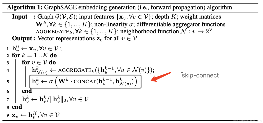

上述前向算法流程中，若干数学符号可解释如下：

• ：表示graph，V表示节点集合，E表示边集合
• ：表示节点 的特征
• ：表示网络深度， 越大，能聚合节点周围更远的邻居信息，可以理解为类似于CNN中卷积的感受野越大。
• ：表示第 层的待学习参数（这里假设该参数已经学习得到）
• ：表示节点 的邻居节点 ，论文中提出是采样节点 周围size个邻居，控制计算复杂度。
• ：表示节点 在第 层的输出
• ：表示第 层的聚合函数（这里假设聚合函数已固定）

上述算法流程核心思想很简单，就是：随着迭代次数的增加(K增加），节点能聚合与他更远的邻居节点的信息。 从而获得节点最终的embedding向量，可供下游任务使用。

上述算法流程的第5行为skip-connect，比较重要

注意：为了使上述算法适用于minibatch方式，可给定一组输入节点，先存好这些节点的邻居节点集合（根据 大小确定采样远近），然后进行上述算法的迭代循环。

一定注意，这里模型输入的是部分节点，而不是整张图和所有节点

注意：由上述算法流程中的第4行可知， 层节点的表示，均由 层的其邻居节点聚合而来，而与本层的邻居节点无关。

邻居节点的定义

为了控制时间复杂度，和适用于minibatch的训练方式，论文提出对节点的邻居节点进行均匀采样时，固定好采样个数，例如对每个输入节点，采样其 个邻居节点( 表示网络的第 层， 表示在 层均匀采样的邻居个数），使得batch每个样本（行）大小一致，方便其送到GPU进行批计算。

论文中提到，实验发现， ， 时效果不错。

GraphSAGE模型的参数学习

这里需要学习的是 ，这里假设 聚合函数是已经选定好了的。

无监督式的：上式中 表示节点 的表征， 表示节点 均匀采样到的邻居节点， 表示sigmoid函数， 表示负采样分布， 表示负采样数量，该损失函数的核心思想就是：使得在graph上距离越近的节点，得到的表征越相似，反之越远越不相似。 与Deepwalk不同，这里的embedding获取是由邻居节点聚合而来。

上述这种无监督的训练得到的节点embedding，一般用作下游任务。

有监督式的：也可以直接在图的训练上接一个特定的任务，例如节点分类任务，则损失函数就为 ，就可以进行端到端的学习和训练。

聚合函数选择

因为节点的邻居节点是没有顺序的，故理想情况下，聚合函数最好对样本的输入时无序的，也就是对输入顺序无要求。论文中提出了以下三种聚合函数。

• Mean aggregator 我们将 Embedding generation algorithm 算法流程中第四行和第五行替换为如下：上式数学公式表达的传播规则和GCN^[9]框架中使用的传播规则极其相似。GCN传播规则如下式：论文中称这种修改后的聚合函数是convolutional的，与论文中其他聚合函数相比，修改后的聚合函数 缺少了Embedding generation algorithm 算法流程中的第5行，聚合时未concat上一层节点本身的 与 聚合的邻居向量 。原始的算法流程中，会concat上一层节点本身的 与 聚合的邻居向量 ，这种拼接操作可以看作一个是GraphSAGE算法在不同的搜索深度或层之间的简单的skip connection，类似于ResNet的形式，它使得模型获得了巨大的提升。

• LSTM aggregator 相对于上面讲到的Mean aggregator，LSTM aggregator表达能力更强，但是是非对称的，需要将邻居节点变成有序的序列。

• Pooling aggregator相当于将每个邻居节点各自独立的扔给一个全连接，这里需要注意 是在特征维度上取最大值。所有邻居节点的权重向量 共享。

注意：上述聚合函数中，除了Mean aggregator 没有Embedding generation algorithm 算法流程中的第5行，其他的聚合函数都有这一步skip connection。

上述这种skip connection的聚合方式可形象的理解为如下图：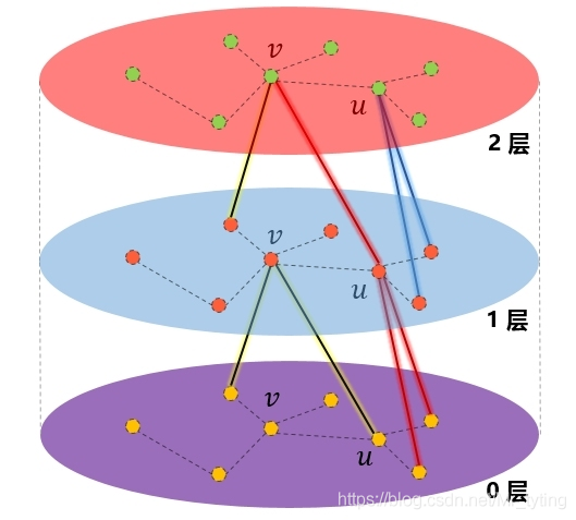

GraphSAGE(Mean aggregator) 与 GCN比较

这里的GCN值得是 paper^[10]

• 从数学公式上看两者的传播规则及其相似。
• GCN是半监督的，是 transductive式的，训练和预测阶段输入的都是整张图和所有节点，即在所有节点上进行传播和学习（对节点及其所有邻居节点，无采样过程），无法应用到新的图上。这里学习到的是所有节点的embedding向量。
• 而GraphSAGE是 inductive 式的，模型的输入只是要节点及其采样的邻居节点集合即可，无需将整张图输入给模型，学习的是一种聚合方式，而非节点的embedding向量，因此学习到了合适的聚合方式，可以快速应用到新的图上。

实验

实验中，我们对训练过程中未见过的节点和图进行预测和测试，对比GraphSAGE与其他的一些方法进行效果比较，同时比较各个聚合函数的实验效果。

分类实验效果如下：

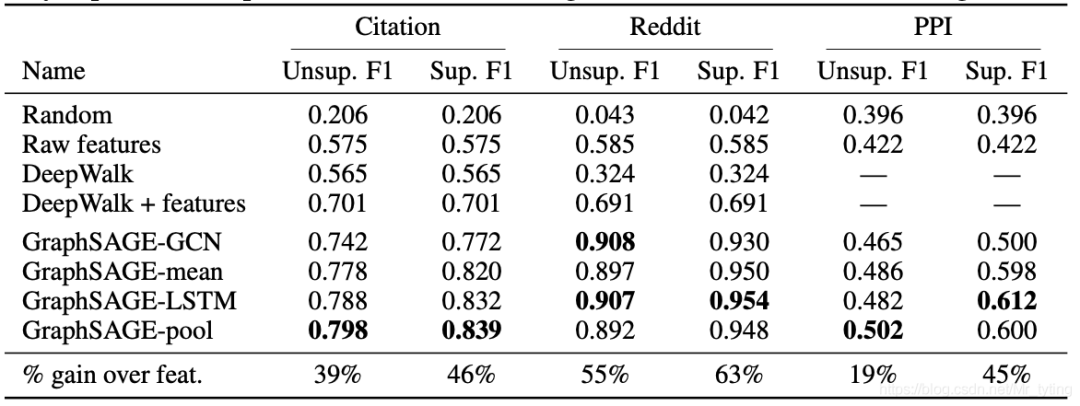上图中的Random、Raw features、Deepwalk、DeepWalk + feature 为一些baseline方法；GraphSAGE-GCN即为本论文提出的mean-aggregator，注意没有skip connection，而GraphSAGE-mean有进行skip connection。

可以看出 ：整体看出，虽然LSTM是非对称的，但是LSTM比pool要好，有监督比无监督要好一些。

运行效率对比

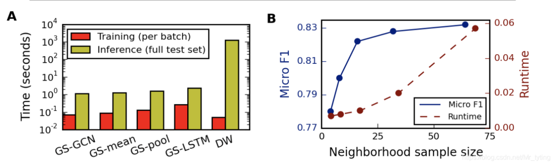可以看出，Graph-GCN耗时最少，Graph-LSTM耗时最多，但是都比Deepwalk耗时低许多；K=2时，邻居节点采样数量在20-25之间效果最好。

核心代码分析

参考的代码链接 graphsage-simple^[11]

数据预处理

两份原始数据集个税如下：

• cora.cites 每行格式如：ID of cited paper \t ID of citing paper

• cora.content 每行格式如：paper_id  word_attributes class_label

def load_cora():
    num_nodes = 2708
    num_feats = 1433
    feat_data = np.zeros((num_nodes, num_feats))
    labels = np.empty((num_nodes,1), dtype=np.int64)
    node_map = {}
    label_map = {}
    with open("cora/cora.content") as fp:
        for i,line in enumerate(fp):
            info = line.strip().split()
            feat_data[i,:] = map(float, info[1:-1])
            node_map[info[0]] = i
            if not info[-1] in label_map:
                label_map[info[-1]] = len(label_map)
            labels[i] = label_map[info[-1]]

    adj_lists = defaultdict(set)
    with open("cora/cora.cites") as fp:
        for i,line in enumerate(fp):
            info = line.strip().split()
            paper1 = node_map[info[0]]
            paper2 = node_map[info[1]]
            adj_lists[paper1].add(paper2)
            adj_lists[paper2].add(paper1)
    return feat_data, labels, adj_lists

得到feat_data 表示 每个节点的初始特征；labels 表示每个节点的标签；adj_lists表示邻接矩阵。

features = nn.Embedding(2708, 1433)
features.weight = nn.Parameter(torch.FloatTensor(feat_data), requires_grad=False)

为所有节点生成一个初始的参数矩阵。注意这里只是初始化，而不是将所有节点喂给模型，等要训练时，只需要从中提取对应的节点即可。

MeanAggregator

class MeanAggregator(nn.Module):
    """
    Aggregates a node's embeddings using mean of neighbors' embeddings
    """
    def __init__(self, features, cuda=False, gcn=False):
        """
        Initializes the aggregator for a specific graph.

        features -- function mapping LongTensor of node ids to FloatTensor of feature values.
        cuda -- whether to use GPU
        gcn --- whether to perform concatenation GraphSAGE-style, or add self-loops GCN-style
        """

        super(MeanAggregator, self).__init__()

        self.features = features
        self.cuda = cuda
        self.gcn = gcn

    def forward(self, nodes, to_neighs, num_sample=10):
        """
        nodes --- list of nodes in a batch
        to_neighs --- list of sets, each set is the set of neighbors for node in batch
        num_sample --- number of neighbors to sample. No sampling if None.
        """
        # Local pointers to functions (speed hack)
        _set = set
        if not num_sample is None:
            _sample = random.sample
            samp_neighs = [_set(_sample(to_neigh,
                            num_sample,
                            )) if len(to_neigh) >= num_sample else to_neigh for to_neigh in to_neighs]
        else:
            samp_neighs = to_neighs

        if self.gcn:
            samp_neighs = [samp_neigh + set([nodes[i]]) for i, samp_neigh in enumerate(samp_neighs)]
        unique_nodes_list = list(set.union(*samp_neighs))
        unique_nodes = {n:i for i,n in enumerate(unique_nodes_list)}
        mask = Variable(torch.zeros(len(samp_neighs), len(unique_nodes)))
        column_indices = [unique_nodes[n] for samp_neigh in samp_neighs for n in samp_neigh]
        row_indices = [i for i in range(len(samp_neighs)) for j in range(len(samp_neighs[i]))]
        mask[row_indices, column_indices] = 1
        if self.cuda:
            mask = mask.cuda()
        num_neigh = mask.sum(1, keepdim=True)
        mask = mask.div(num_neigh)
        if self.cuda:
            embed_matrix = self.features(torch.LongTensor(unique_nodes_list).cuda())
        else:
            embed_matrix = self.features(torch.LongTensor(unique_nodes_list))
        to_feats = mask.mm(embed_matrix)
        return to_feats

上述代码可理解为Embedding generation algorithm 算法流程中的 第4行。

其中num_sample表示对邻居节点采样， self.features 表示 节点的初始特征向量，nodes表示参与训练或预测的节点；如果是mean-GCN模式，则节点的邻居节点包括节点本身，其中mask矩阵表示归一化后的邻接矩阵，embed_matrix表示节点在上一层的输出；mask.mm(embed_matrix)则为聚合后结果。

encoder

class Encoder(nn.Module):
    """
    Encodes a node's using 'convolutional' GraphSage approach
    """
    def __init__(self, features, feature_dim,
            embed_dim, adj_lists, aggregator,
            num_sample=10,
            base_model=None, gcn=False, cuda=False,
            feature_transform=False):
        super(Encoder, self).__init__()

        self.features = features
        self.feat_dim = feature_dim
        self.adj_lists = adj_lists
        self.aggregator = aggregator
        self.num_sample = num_sample
        if base_model != None:
            self.base_model = base_model

        self.gcn = gcn
        self.embed_dim = embed_dim
        self.cuda = cuda
        self.aggregator.cuda = cuda
        self.weight = nn.Parameter(
                torch.FloatTensor(embed_dim, self.feat_dim if self.gcn else 2 * self.feat_dim))
        init.xavier_uniform(self.weight)

    def forward(self, nodes):
        """
        Generates embeddings for a batch of nodes.

        nodes     -- list of nodes
        """
        neigh_feats = self.aggregator.forward(nodes, [self.adj_lists[int(node)] for node in nodes],
                self.num_sample)
        if not self.gcn:
            if self.cuda:
                self_feats = self.features(torch.LongTensor(nodes).cuda())
            else:
                self_feats = self.features(torch.LongTensor(nodes))
            combined = torch.cat([self_feats, neigh_feats], dim=1)
        else:
            combined = neigh_feats
        combined = F.relu(self.weight.mm(combined.t()))
        return combined

上述代码可理解为Embedding generation algorithm 算法流程中的 第4行和第5行，先调用aggregator进行聚合，在进行concat。其中nodes表示参与训练或预测的节点；当是GCN模式时，无需concat节点上一层输出，反之则需要。

模型训练和预测

    graphsage = SupervisedGraphSage(3, enc2)
#    graphsage.cuda()
    rand_indices = np.random.permutation(num_nodes)
    test = rand_indices[:1000]
    val = rand_indices[1000:1500]
    train = list(rand_indices[1500:])

    optimizer = torch.optim.SGD(filter(lambda p : p.requires_grad, graphsage.parameters()), lr=0.7)
    times = []
    for batch in range(200):
        batch_nodes = train[:1024]
        random.shuffle(train)
        start_time = time.time()
        optimizer.zero_grad()
        loss = graphsage.loss(batch_nodes,
                Variable(torch.LongTensor(labels[np.array(batch_nodes)])))
        loss.backward()
        optimizer.step()
        end_time = time.time()
        times.append(end_time-start_time)
        print batch, loss.data[0]

    val_output = graphsage.forward(val)
    print "Validation F1:", f1_score(labels[val], val_output.data.numpy().argmax(axis=1), average="micro")
    print "Average batch time:", np.mean(times)

从上面代码可以看出，模型训练和预测时，输入的只是不同节点及其对应邻居节点即可，不需要输入整张图和所有节点。

个人总结

• 其实GraphSAGE与GCN中传播规则几乎一样，但是一个是transductive式，一个inductive式，区别体现在邻居节点采样和训练目的上，GraphSAGE对邻居节点进行均匀采样，目的是学习一种聚合方式；而GCN则可理解为对节点的所有邻居节点聚合，学习的是所有节点的embedding。

参考资料