


1、导入模块
1import cf
2import cfplot as cfp
3import warnings
4warnings.filterwarnings('ignore')复制
2、采样方法
Read in a precipitation field and inspect it
1f1 = cf.read('ncas_data/precip_2010.nc')[0]
2print(f1)复制
output:
1Field: long_name=precipitation (ncvar%pre)
2------------------------------------------
3Data : long_name=precipitation(long_name=time(12), latitude(145), longitude(53)) mm
4Dimension coords: long_name=time(12) = [2010-01-16 00:00:00, ..., 2010-12-16 00:00:00] gregorian
5 : latitude(145) = [-90.0, ..., 90.0] degrees_north
6 : longitude(53) = [-33.75, ..., 63.75] degrees_east复制
Read in another, lower-resolution, precipitation field and inspect it
1g1 = cf.read('ncas_data/model_precip_DJF_means_low_res.nc')[0]
2print(g1)复制
output:
1Field: long_name=precipitation (ncvar%precip)
2---------------------------------------------
3Data : long_name=precipitation(long_name=t(1), long_name=Surface(1), latitude(73), longitude(27)) mm/day
4Cell methods : long_name=t(1): mean
5Dimension coords: long_name=t(1) = [1996-07-16 00:00:00] 360_day
6 : long_name=Surface(1) = [0.0] level
7 : latitude(73) = [-90.0, ..., 90.0] degrees_north
8 : longitude(27) = [-33.75, ..., 63.75] degrees_east复制
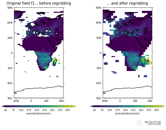
Regrid the first field to the grid of the second and inspect the results
1h1 = f1.regrids(g1, method='conservative')
2print(h1)复制
output:
1Field: long_name=precipitation (ncvar%pre)
2------------------------------------------
3Data : long_name=precipitation(long_name=time(12), latitude(73), longitude(27)) mm
4Dimension coords: long_name=time(12) = [2010-01-16 00:00:00, ..., 2010-12-16 00:00:00] gregorian
5 : latitude(73) = [-90.0, ..., 90.0] degrees_north
6 : longitude(27) = [-33.75, ..., 63.75] degrees_east复制
Plot before and after
1cfp.gopen(rows=1, columns=2)
2cfp.gpos(1)
3cfp.con(f1[0], blockfill=True, lines=False, colorbar_label_skip=2,
4 title='Original field f1... before regridding')
5cfp.gpos(2)
6cfp.con(h1[0], blockfill=True, lines=False, colorbar_label_skip=2,
7 title='... and after regridding')
8cfp.gclose()复制
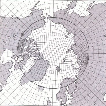
(2)三极网格(tripolar grid)采样
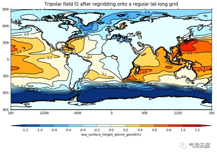
Read in and inspect a sea surface height field contained on a tripolar grid
1f2 = cf.read('ncas_data/tripolar.nc')[0]
2print(f2)复制
output:
1Field: sea_surface_height_above_geoid (ncvar%sossheig)
2------------------------------------------------------
3Data : sea_surface_height_above_geoid(time(1), ncdim%y(332), ncdim%x(362)) m
4Cell methods : time(1): mean (interval: 2700 s)
5Dimension coords: time(1) = [1978-09-06 00:00:00] 360_day
6Auxiliary coords: time(time(1)) = [1978-09-06 00:00:00] 360_day
7 : longitude(ncdim%y(332), ncdim%x(362)) = [[72.5, ..., 72.98915100097656]] degrees_east
8 : latitude(ncdim%y(332), ncdim%x(362)) = [[-84.21070861816406, ..., 50.01094055175781]] degrees_north复制
Read in a field (precipitation, but not relevant) defined on a regular lat-long grid
1g2 = cf.read('ncas_data/model_precip_DJF_means.nc')[0]
2print(g2)复制
output:
1Field: long_name=precipitation (ncvar%precip)
2---------------------------------------------
3Data : long_name=precipitation(long_name=t(1), long_name=Surface(1), latitude(145), longitude(192)) mm/day
4Cell methods : long_name=t(1): mean
5Dimension coords: long_name=t(1) = [1996-07-16 00:00:00] 360_day
6 : long_name=Surface(1) = [0.0] level
7 : latitude(145) = [-90.0, ..., 90.0] degrees_north
8 : longitude(192) = [0.0, ..., 358.125] degrees_east复制
Regrid the field on the tripolar grid to the regular lat-long grid
1h2 = f2.regrids(g2, method='bilinear', src_axes={'X': 'ncdim%x', 'Y': 'ncdim%y'},
2 src_cyclic=True)
3print(h2)复制
output:
1Field: sea_surface_height_above_geoid (ncvar%sossheig)
2------------------------------------------------------
3Data : sea_surface_height_above_geoid(time(1), latitude(145), longitude(192)) m
4Cell methods : time(1): mean (interval: 2700 s)
5Dimension coords: time(1) = [1978-09-06 00:00:00] 360_day
6 : latitude(145) = [-90.0, ..., 90.0] degrees_north
7 : longitude(192) = [0.0, ..., 358.125] degrees_east
8Auxiliary coords: time(time(1)) = [1978-09-06 00:00:00] 360_day复制
Plot the regridded data
1cfp.levs(min=-1.2, max=1.2, step=0.2)
2cfp.con(h2, title='Tripolar field f2 after regridding onto a regular lat-long grid')复制
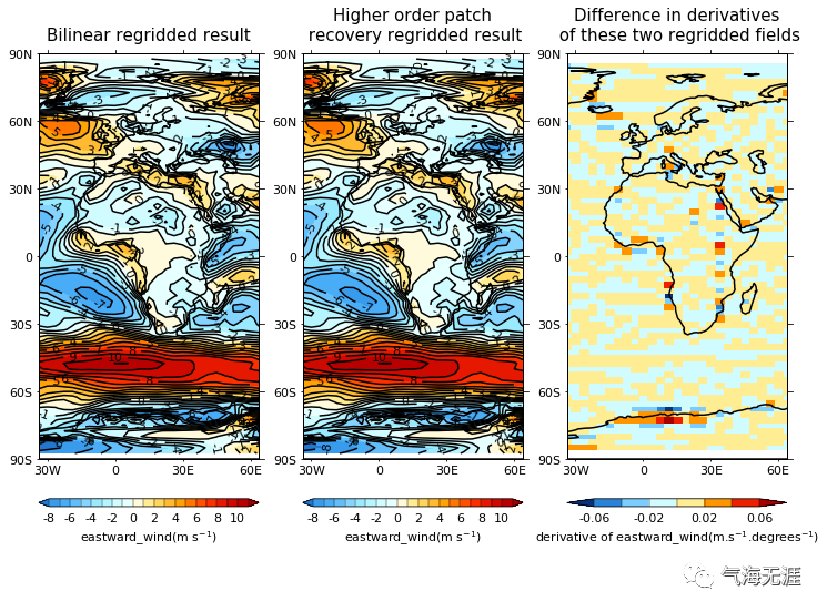
(3)不同采样方法比较
Read in a wind field and inspect it
1f3 = cf.read('ncas_data/data5.nc')[0].subspace[0, 0]
2print(f3)复制
output:
1Field: eastward_wind (ncvar%U)
2------------------------------
3Data : eastward_wind(time(1), pressure(1), latitude(160), longitude(320)) m s**-1
4Dimension coords: time(1) = [1987-03-15 00:00:00]
5 : pressure(1) = [1000.0] mbar
6 : latitude(160) = [89.14151763916016, ..., -89.14151763916016] degrees_north
7 : longitude(320) = [0.0, ..., 358.875] degrees_east复制
Visualise this original wind field
1cfp.levs()
2cfp.cscale()
3cfp.con(f3, title='Original field f3 (i.e. before regridding)')复制

Read in another field (precipitation, but the nature is not relevant) and inspect it
1g3 = cf.read('ncas_data/model_precip_DJF_means_low_res.nc')[0]
2print(g3)复制
output:
1Field: long_name=precipitation (ncvar%precip)
2---------------------------------------------
3Data : long_name=precipitation(long_name=t(1), long_name=Surface(1), latitude(73), longitude(27)) mm/day
4Cell methods : long_name=t(1): mean
5Dimension coords: long_name=t(1) = [1996-07-16 00:00:00] 360_day
6 : long_name=Surface(1) = [0.0] level
7 : latitude(73) = [-90.0, ..., 90.0] degrees_north
8 : longitude(27) = [-33.75, ..., 63.75] degrees_east复制
Regrid the first field to the grid of the second using bilinear interpolation
1h3 = f3.regrids(g3, method='bilinear')
2print(h3)复制
output:
1Field: eastward_wind (ncvar%U)
2------------------------------
3Data : eastward_wind(time(1), pressure(1), latitude(73), longitude(27)) m s**-1
4Dimension coords: time(1) = [1987-03-15 00:00:00]
5 : pressure(1) = [1000.0] mbar
6 : latitude(73) = [-90.0, ..., 90.0] degrees_north
7 : longitude(27) = [-33.75, ..., 63.75] degrees_east复制
Regrid the first field to the grid of the second using higher order patch recovery
1i3 = f3.regrids(g3, method='patch')
2print(i3)复制
output:
1Field: eastward_wind (ncvar%U)
2------------------------------
3Data : eastward_wind(time(1), pressure(1), latitude(73), longitude(27)) m s**-1
4Dimension coords: time(1) = [1987-03-15 00:00:00]
5 : pressure(1) = [1000.0] mbar
6 : latitude(73) = [-90.0, ..., 90.0] degrees_north
7 : longitude(27) = [-33.75, ..., 63.75] degrees_east复制
Find the Y derivatives of the regridded fields
1deriv_h = h3.derivative('Y')
2deriv_h.units = 'm.s-1.degrees-1'
3deriv_i = i3.derivative('Y')
4deriv_i.units = 'm.s-1.degrees-1'复制
Plot the regridded fields and the differences between their derivatives
1cfp.gopen(rows=1, columns=3)
2cfp.gpos(1)
3cfp.con(h3, colorbar_label_skip=2, title='Bilinear regridded result')
4cfp.gpos(2)
5cfp.con(i3, colorbar_label_skip=2,
6 title='Higher order patch\n recovery regridded result')
7cfp.gpos(3)
8cfp.levs(min=-0.06, max=0.06, step=0.02)
9cfp.cscale('scale1')
10cfp.con(deriv_i - deriv_h, blockfill=True, lines=False, colorbar_label_skip=2,
11 title='Difference in derivatives\n of these two regridded fields')
12cfp.gclose()复制
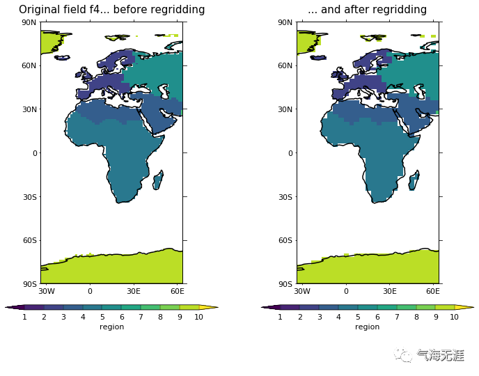
(4)最近邻采样法(the nearest neighbour method)
Read in a region field and inspect it
1f4 = cf.read('ncas_data/regions.nc')[0]
2print(f4)复制
output:
1Field: region (ncvar%Regionmask)
2--------------------------------
3Data : region(latitude(145), longitude(53))
4Dimension coords: latitude(145) = [-90.0, ..., 90.0] degrees_north
5 : longitude(53) = [-33.75, ..., 63.75] degrees_east复制
Read in another field (precipitation, but the nature is not relevant) and inspect it
1g4 = cf.read('ncas_data/model_precip_DJF_means_low_res.nc')[0]
2print(g4)复制
output:
1Field: long_name=precipitation (ncvar%precip)
2---------------------------------------------
3Data : long_name=precipitation(long_name=t(1), long_name=Surface(1), latitude(73), longitude(27)) mm/day
4Cell methods : long_name=t(1): mean
5Dimension coords: long_name=t(1) = [1996-07-16 00:00:00] 360_day
6 : long_name=Surface(1) = [0.0] level
7 : latitude(73) = [-90.0, ..., 90.0] degrees_north
8 : longitude(27) = [-33.75, ..., 63.75] degrees_east复制
Regrid using nearest source to destination regridding and inspect the result
1h4 = f4.regrids(g4, method='nearest_stod')
2print(h4)复制
output:
1Field: region (ncvar%Regionmask)
2--------------------------------
3Data : region(latitude(73), longitude(27))
4Dimension coords: latitude(73) = [-90.0, ..., 90.0] degrees_north
5 : longitude(27) = [-33.75, ..., 63.75] degrees_east复制
Plot before and after
1cfp.gopen(rows=1, columns=2)
2cfp.levs(min=1, max=10, step=1)
3cfp.cscale()
4cfp.gpos(1)
5cfp.con(
6 f4, blockfill=True, lines=False, title='Original field f4... before regridding')
7cfp.gpos(2)
8cfp.con(h4, blockfill=True, lines=False, title='... and after regridding')
9cfp.gclose()复制
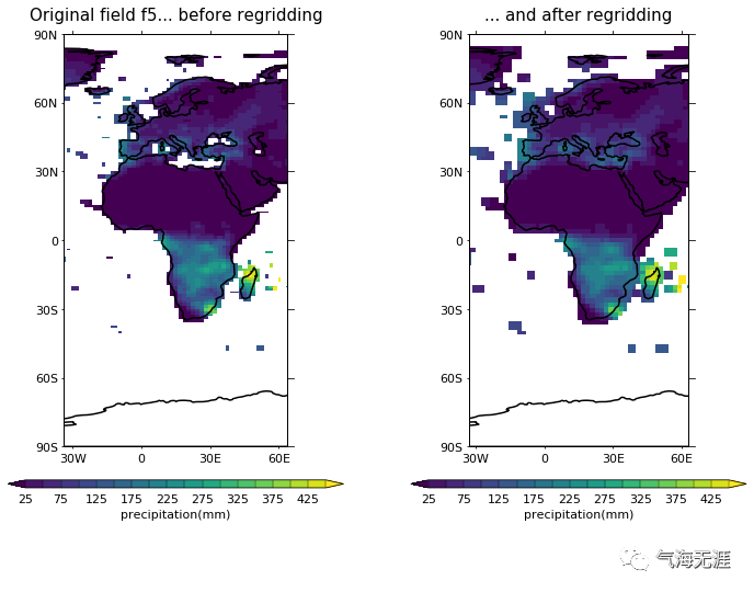
(5)网格分辨率采样
Read in a precipitation field and inspect it
1f5 = cf.read('ncas_data/precip_2010.nc')[0]
2print(f5)复制
output:
1Field: long_name=precipitation (ncvar%pre)
2------------------------------------------
3Data : long_name=precipitation(long_name=time(12), latitude(145), longitude(53)) mm
4Dimension coords: long_name=time(12) = [2010-01-16 00:00:00, ..., 2010-12-16 00:00:00] gregorian
5 : latitude(145) = [-90.0, ..., 90.0] degrees_north
6 : longitude(53) = [-33.75, ..., 63.75] degrees_east复制
Create dimension coordinates for the destination grid
1import numpy as np
2lon = cf.DimensionCoordinate(data=cf.Data(np.arange(-33, 64, 2.0), 'degrees_east'))
3lat = cf.DimensionCoordinate(data=cf.Data(np.arange(-90, 91, 2.0), 'degrees_north'))复制
Create Voronoi bounds for the new dimension coordinates
1lon_bounds = lon.create_bounds()
2lat_bounds = lat.create_bounds(min=-90, max=90)
3lon.set_bounds(lon_bounds)
4lat.set_bounds(lat_bounds)复制
Regrid field onto the grid of the new coordinates conservatively and inspect the result
1g5 = f5.regrids({'longitude': lon, 'latitude': lat}, method='conservative')
2print(g5)复制
output:
1Field: long_name=precipitation (ncvar%pre)
2------------------------------------------
3Data : long_name=precipitation(long_name=time(12), latitude(91), longitude(49)) mm
4Dimension coords: long_name=time(12) = [2010-01-16 00:00:00, ..., 2010-12-16 00:00:00] gregorian
5 : latitude(91) = [-90.0, ..., 90.0] degrees_north
6 : longitude(49) = [-33.0, ..., 63.0] degrees_east复制
Plot before and after
1cfp.gopen(rows=1, columns=2)
2cfp.levs()
3cfp.gpos(1)
4cfp.con(f5[0], blockfill=True, lines=False, colorbar_label_skip=2,
5 title='Original field f5... before regridding')
6cfp.gpos(2)
7cfp.con(g5[0], blockfill=True, lines=False, colorbar_label_skip=2,
8 title='... and after regridding')
9cfp.gclose()复制
(6)时间序列采样
Read in a precipitation field and inspect it
1f6 = cf.read('ncas_data/precip_1D_yearly.nc')[0]
2print(f6)复制
output:
1Field: long_name=precipitation (ncvar%pre)
2------------------------------------------
3Data : long_name=precipitation(long_name=time(10), long_name=latitude(1), long_name=longitude(1)) mm
4Cell methods : long_name=time(10): mean long_name=latitude(1): long_name=longitude(1): mean
5Dimension coords: long_name=time(10) = [1981-07-02 00:00:00, ..., 1990-07-02 00:00:00] gregorian
6 : long_name=latitude(1) = [0.0] degrees_north
7 : long_name=longitude(1) = [0.0] degrees_east复制
Read in another precipitation field, with more time axis points, and inspect it
1g6 = cf.read('ncas_data/precip_1D_monthly.nc')[0]
2print(g6)复制
output:
1Field: long_name=precipitation (ncvar%pre)
2------------------------------------------
3Data : long_name=precipitation(long_name=time(120), long_name=latitude(1), long_name=longitude(1)) mm
4Cell methods : long_name=latitude(1): long_name=longitude(1): mean
5Dimension coords: long_name=time(120) = [1981-01-16 00:00:00, ..., 1990-12-16 00:00:00] gregorian
6 : long_name=latitude(1) = [0.0] degrees_north
7 : long_name=longitude(1) = [0.0] degrees_east复制
Regrid linearly along the time axis 'T' and summarise the resulting field
1h6 = f6.regridc(g6, axes='T', method='bilinear')
2print(h6)复制
output:
1Field: long_name=precipitation (ncvar%pre)
2------------------------------------------
3Data : long_name=precipitation(long_name=time(120), long_name=latitude(1), long_name=longitude(1)) mm
4Cell methods : long_name=time(120): mean long_name=latitude(1): long_name=longitude(1): mean
5Dimension coords: long_name=time(120) = [1981-01-16 00:00:00, ..., 1990-12-16 00:00:00] gregorian
6 : long_name=latitude(1) = [0.0] degrees_north
7 : long_name=longitude(1) = [0.0] degrees_east复制
Plot the time series before and after regridding
1cfp.gopen(rows=1, columns=2)
2cfp.gpos(1)
3cfp.lineplot(f6, marker='o', color='red',
4 title='Original time series... before regridding')
5cfp.gpos(2)
6cfp.lineplot(h6, marker='o', color='blue', title='... and after regridding')
7cfp.gclose()复制

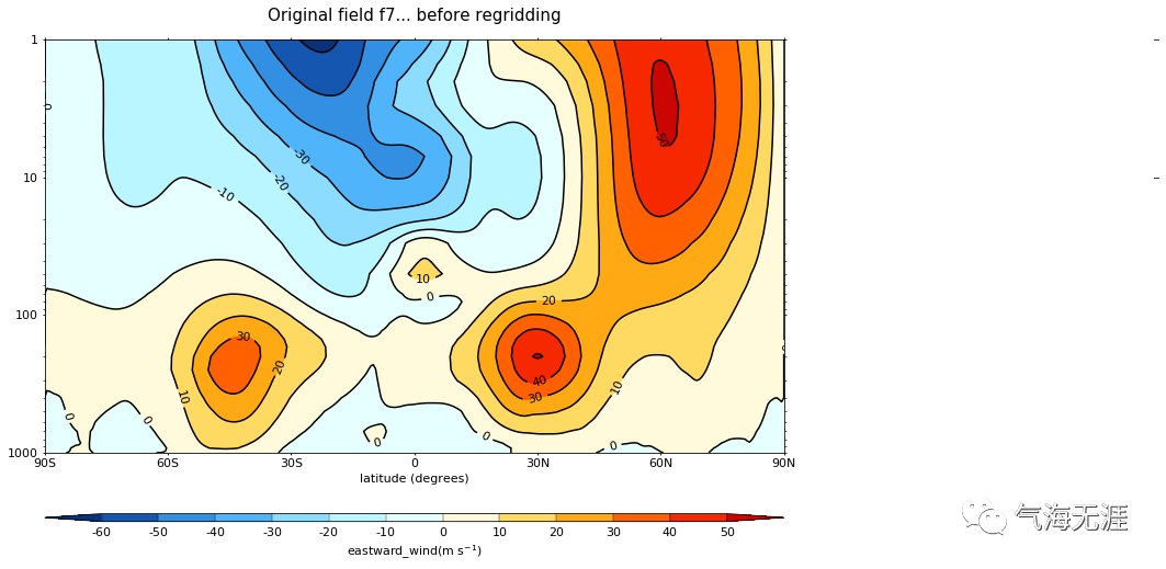
(7)垂直采样
Read in a wind field and inspect it
1f7 = cf.read('ncas_data/u_n216.nc')[0]
2print(f7)复制
output:
1Field: eastward_wind (ncvar%u)
2------------------------------
3Data : eastward_wind(long_name=t(1), long_name=Pressure(39), latitude(325), longitude(1)) m s-1
4Dimension coords: long_name=t(1) = [1850-01-16 00:00:00] 360_day
5 : long_name=Pressure(39) = [1000.0, ..., 0.029999999329447746] mbar
6 : latitude(325) = [-90.0, ..., 90.00000762939453] degrees_north
7 : longitude(1) = [358.33331298828125] degrees_east复制
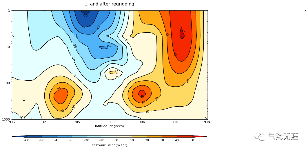
Read in another, lower-resolution, wind field and inspect it
1g7 = cf.read('ncas_data/u_n96.nc')[0]
2print(g7)复制
output:
1Field: eastward_wind (ncvar%u)
2------------------------------
3Data : eastward_wind(long_name=t(1), air_pressure(19), latitude(145), longitude(1)) m s-1
4Dimension coords: long_name=t(1) = [1850-01-16 00:00:00] 360_day
5 : air_pressure(19) = [1000, ..., 1] mbar
6 : latitude(145) = [-90.0, ..., 90.0] degrees_north
7 : longitude(1) = [356.25] degrees_east复制
Save the pressure coordinates and their keys
1p_src = f7.coordinate('Z').copy()
2p_dst = g7.coordinate('Z').copy()复制
Take the log of the pressures
1f7.coordinate('Z').log(base=10, inplace=True)
2g7.coordinate('Z').log(base=10, inplace=True)复制
Regrid the source field and inspect the result
1h7 = f7.regridc(g7, axes=('Y', 'Z'), method='bilinear')
2print(h7)复制
output:
1Field: eastward_wind (ncvar%u)
2------------------------------
3Data : eastward_wind(long_name=t(1), ncdim%air_pressure(19), latitude(145), longitude(1)) m s-1
4Dimension coords: long_name=t(1) = [1850-01-16 00:00:00] 360_day
5 : ncvar%air_pressure(ncdim%air_pressure(19)) = [6.907755278982137, ..., 0.0] ln(re 100 Pa)
6 : latitude(145) = [-90.0, ..., 90.0] degrees_north
7 : longitude(1) = [358.33331298828125] degrees_east复制
Insert the saved destination pressure coordinate into the regridded field
1h7.replace_construct('Z', p_dst)
2print(h7)复制
output:
1Field: eastward_wind (ncvar%u)
2------------------------------
3Data : eastward_wind(long_name=t(1), air_pressure(19), latitude(145), longitude(1)) m s-1
4Dimension coords: long_name=t(1) = [1850-01-16 00:00:00] 360_day
5 : air_pressure(19) = [1000, ..., 1] mbar
6 : latitude(145) = [-90.0, ..., 90.0] degrees_north
7 : longitude(1) = [358.33331298828125] degrees_east复制
Reinsert the saved pressure coordinates into the original fields
1f7.replace_construct('Z', p_src)
2g7.replace_construct('Z', p_dst)复制
Plot before and after
1cfp.con(f7, title='Original field f7... before regridding', ylog=True)
2cfp.con(g7, title='... and after regridding', ylog=True)复制
有问题可以到QQ群里进行讨论,我们在那边等大家。
QQ群号:854684131
