Python气象数据处理与绘图：集合经验模态分解（EEMD）

1、导入模块

1from PyEMD import EMD, EEMD
2from PyEMD.visualisation import Visualisation 
3import numpy  as np
4import pylab as plt
5
6import warnings
7warnings.filterwarnings('ignore')

复制

2、经验模态分解（EMD）

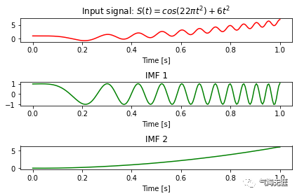
相对于小波分解，EMD具有自适性、后验性，并能对信号进行平稳化处理，在气象要素分析及实际业务中被广泛应用，可用于发展新的预测方法和集合预报技术。EMD算法能将原始信号不断进行分解，获取符合一定条件下的IMF分量。这些 IMF 分量之间的频率往往不同，这就为其在谐波检测方向的使用提供了一种思路。

 1# Define signal
 2t = np.linspace(0, 1, 200)
 3s = np.cos(11*2*np.pi*t*t) + 6*t*t
 4
 5# Execute EMD on signal
 6IMF = EMD().emd(s,t)
 7N = IMF.shape[0]+1
 8
 9# Plot results
10plt.subplot(N,1,1)
11plt.plot(t, s, 'r')
12plt.title("Input signal: $S(t)=cos(22\pi t^2) + 6t^2$")
13plt.xlabel("Time [s]")
14
15for n, imf in enumerate(IMF):
16    plt.subplot(N,1,n+2)
17    plt.plot(t, imf, 'g')
18    plt.title("IMF "+str(n+1))
19    plt.xlabel("Time [s]")
20
21plt.tight_layout()
22plt.show()

复制

3、集合经验模态分解（EEMD）

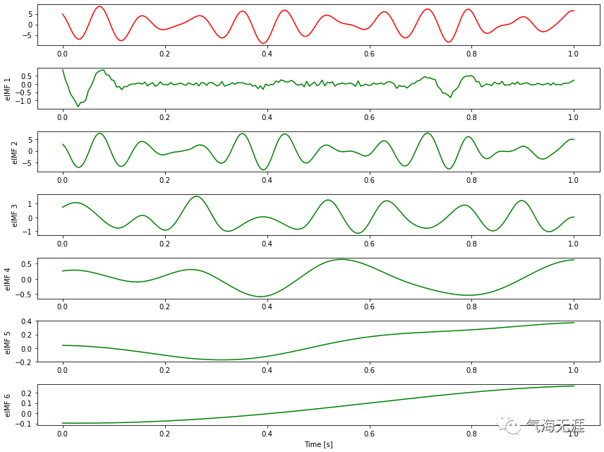
EMD 算法以其正交性、收敛性等特点被广泛用于信号处理等领域，但并不像小波分析或者神经网络那样，有固定的数学模型，因此它的一些重要性质仍还没有通过缜密的数学方法证明出。而且对模态分量 IMF 的定义也尚未统一，仅能从信号的零点与极值点的联系与信号的局部特征等综合描述。

EMD在信号分析中存在一定缺陷——尺度混合，导致分解在物理上不唯一，甚至失去意义。为了弥补尺度混合等问题，在其基础上发展了EEMD(Ensemble Empirical Mode Decomposition)。因此，EEMD即继承了EMD自适性等优点，又避免了尺度混合的缺陷。EEMD分解算法基于白噪声频谱均衡的分布特点来均衡噪声，使得频率的分布趋于均匀。添加的白噪声不同信号的幅值分布点带来的模态混叠效应。EEMD分解满足自适应性，其分解结果决定于资料长度本身，与分解次数无关。

 1# Define signal
 2t = np.linspace(0, 1, 200)
 3
 4sin = lambda x,p: np.sin(2*np.pi*x*t+p)
 5S = 3*sin(18,0.2)*(t-0.2)**2
 6S += 5*sin(11,2.7)
 7S += 3*sin(14,1.6)
 8S += 1*np.sin(4*2*np.pi*(t-0.8)**2)
 9S += t**2.1 -t
10
11# Assign EEMD to `eemd` variable
12eemd = EEMD()
13
14# Say we want detect extrema using parabolic method
15emd = eemd.EMD
16emd.extrema_detection="parabol"
17
18# Execute EEMD on S
19eIMFs = eemd.eemd(S, t)
20nIMFs = eIMFs.shape[0]
21
22# Plot results
23plt.figure(figsize=(12,9))
24plt.subplot(nIMFs+1, 1, 1)
25plt.plot(t, S, 'r')
26
27for n in range(nIMFs):
28    plt.subplot(nIMFs+1, 1, n+2)
29    plt.plot(t, eIMFs[n], 'g')
30    plt.ylabel("eIMF %i" %(n+1))
31    plt.locator_params(axis='y', nbins=5)
32
33plt.xlabel("Time [s]")
34plt.tight_layout()
35plt.show()

复制

4、读取海温数据并预处理

1# url = 'http://paos.colorado.edu/research/wavelets/wave_idl/nino3sst.txt'
2# dat = np.genfromtxt(url, skip_header=19)
3dat = np.loadtxt('/home/mw/work/nino3sst.txt',skiprows=19)
4print(dat.shape)

复制

输出：

1(504,)

复制

变量赋值

1t0 = 1871.0                               # 开始的时间，以年为单位
2dt = 0.25                                 # 采样间隔，以年为单位
3N = dat.size                              # 时间序列的长度
4t = np.arange(0, N) * dt + t0             # 构造时间序列数组

复制

数据处理

1p = np.polyfit(t - t0, dat, 1)               # 线性拟合
2dat_notrend = dat - np.polyval(p, t - t0)    # 去趋势
3std = dat_notrend.std()                      # 标准差
4var = std ** 2                               # 方差
5dat_norm = dat_notrend / std                 # 标准化

复制

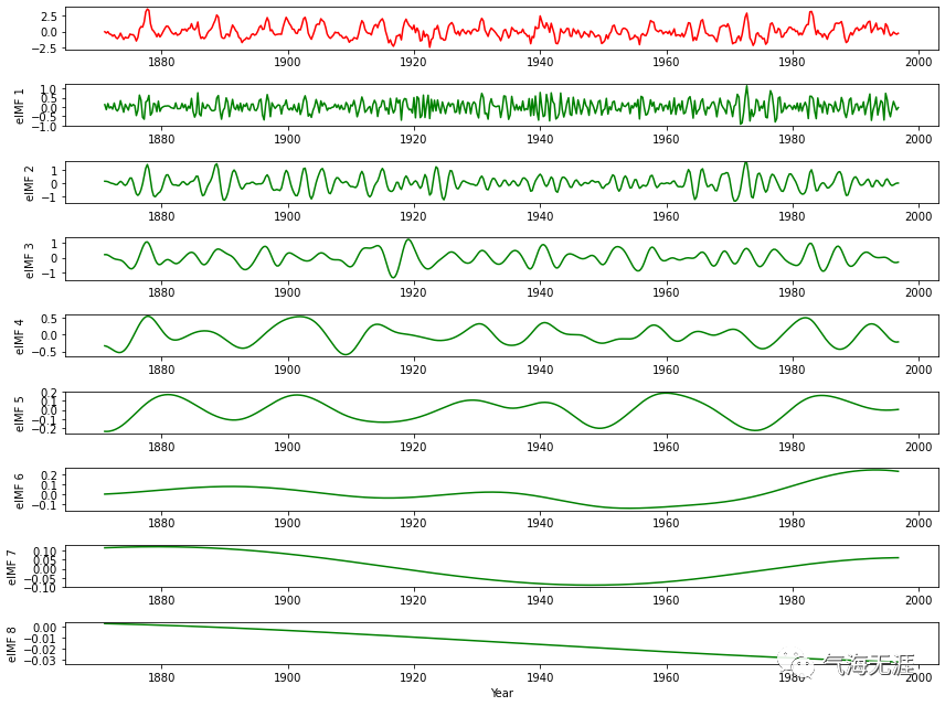
5、nino3海温距平数据的集合经验模态分解

 1# Assign EEMD to `eemd` variable
 2eemd = EEMD()
 3
 4# Say we want detect extrema using parabolic method
 5emd = eemd.EMD
 6#emd.extrema_detection="parabol"
 7
 8# Execute EEMD on S
 9eIMFs = eemd.eemd(dat_norm, t)
10nIMFs = eIMFs.shape[0]
11
12# Plot results
13plt.figure(figsize=(12,9))
14plt.subplot(nIMFs+1, 1, 1)
15plt.plot(t, dat_norm, 'r')
16
17for n in range(nIMFs):
18    plt.subplot(nIMFs+1, 1, n+2)
19    plt.plot(t, eIMFs[n], 'g')
20    plt.ylabel("eIMF %i" %(n+1))
21    plt.locator_params(axis='y', nbins=5)
22
23plt.xlabel("Year")
24plt.tight_layout()
25plt.show()

复制

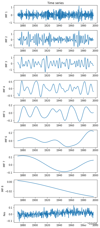
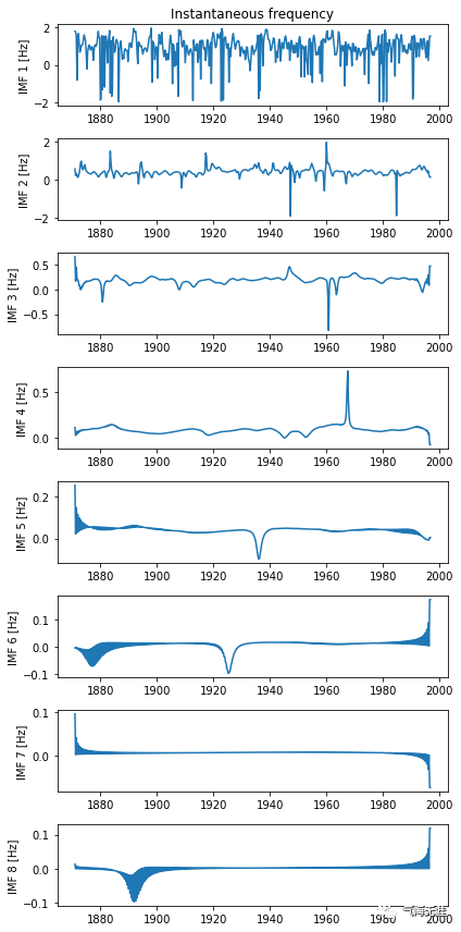
6、绘制IMF和瞬时频率

1imfs, res = eemd.get_imfs_and_residue()
2vis = Visualisation()
3vis.plot_imfs(imfs=imfs, residue=res, t=t, include_residue=True)
4vis.plot_instant_freq(t, imfs=imfs)
5vis.show()
复制