


本文是DEEP LEARNING WITH PYTORCH: A 60 MINUTE BLITZ的学习笔记
这里继续进行第二部分A GENTLE INTRODUCTION TO TORCH.AUTOGRAD:
torch.autograd
is PyTorch’s automatic differentiation engine that powers neural network training. In this section, you will get a conceptual understanding of how autograd helps a neural network train. (自动求导 --- 神经网络训练)
1. Background
Neural networks (NNs) are a collection of nested functions that are executed on some input data. These functions are defined by parameters (consisting of weights and biases), which in PyTorch are stored in tensors.
Training a NN happens in two steps:
Forward Propagation: In forward prop, the NN makes its best guess about the correct output. It runs the input data through each of its functions to make this guess. Backward Propagation: In backprop, the NN adjusts its parameters proportionate to the error in its guess. It does this by traversing backwards from the output, collecting the derivatives of the error with respect to the parameters of the functions (gradients), and optimizing the parameters using gradient descent.
训练神经网络的两步:前向传播&反向传播,反向传播即是误差error(loss)对weights和biases求偏导,不断更新weights和biases,反复迭代的过程。
2. Usage in PyTorch
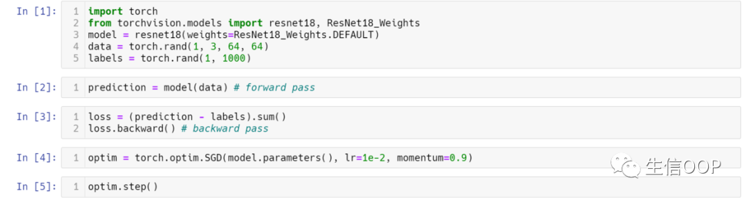
Let’s take a look at a single training step. For this example, we load a pretrained resnet18 model from torchvision. We create a random data tensor to represent a single image with 3 channels, and height & width of 64, and its corresponding label initialized to some random values. Label in pretrained models has shape (1,1000).
加载torchvision中的预训练模型resnet18。随机生成的数据是一个3个通道64×64的图像,label定义为1000个数值。
import torch
from torchvision.models import resnet18, ResNet18_Weights
model = resnet18(weights=ResNet18_Weights.DEFAULT)
data = torch.rand(1, 3, 64, 64)
labels = torch.rand(1, 1000)复制
Next, we run the input data through the model through each of its layers to make a prediction. This is the forward pass. We use the model’s prediction and the corresponding label to calculate the error (loss). The next step is to backpropagate this error through the network. Backward propagation is kicked off when we call .backward()
on the error tensor. Autograd then calculates and stores the gradients for each model parameter in the parameter’s .grad
attribute.
prediction = model(data) # forward pass
loss = (prediction - labels).sum()
loss.backward() # backward pass复制
Next, we load an optimizer, in this case SGD with a learning rate of 0.01 and momentum. Finally, we call .step()
to initiate gradient descent. The optimizer adjusts each parameter by its gradient stored in .grad
.
optim = torch.optim.SGD(model.parameters(), lr=1e-2, momentum=0.9)
optim.step() #gradient descent复制
3. Differentiation in Autograd
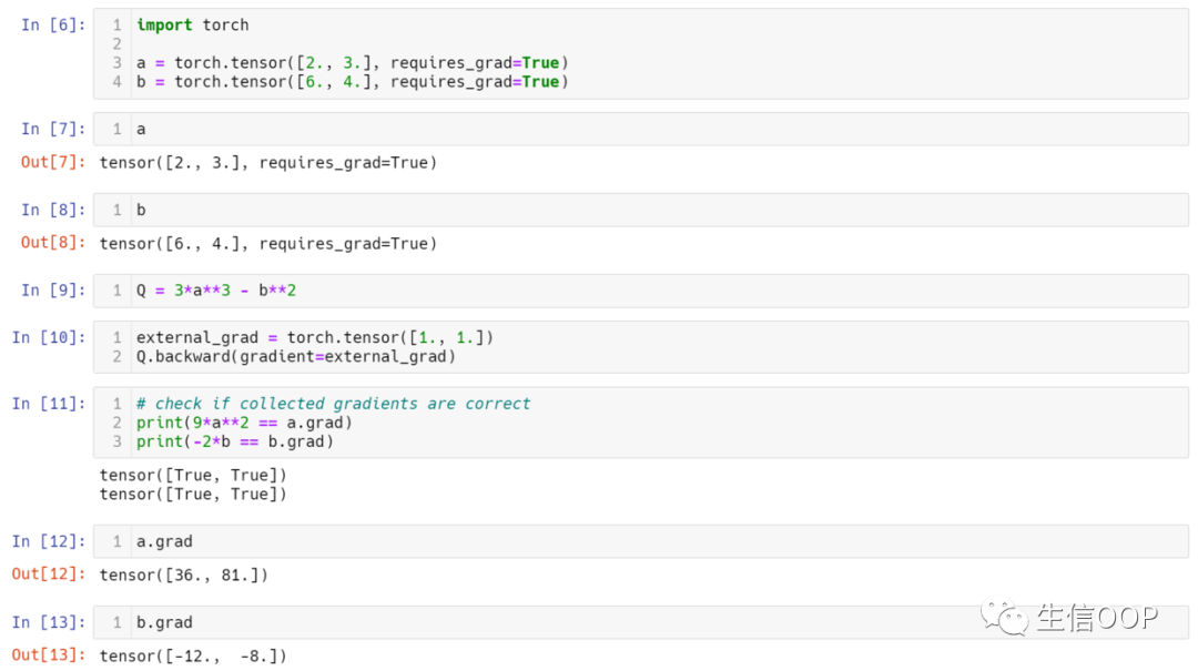
We create two tensors a and b with requires_grad=True
. This signals to autograd
that every operation on them should be tracked. We create another tensor Q from a and b.
import torch
a = torch.tensor([2., 3.], requires_grad=True)
b = torch.tensor([6., 4.], requires_grad=True)
Q = 3*a**3 - b**2复制
对于方法.backward()
而言,如果对应变量是一个标量,则无需传递参数,如果对应变量是一个向量,则必须显式指定一个gradient
参数,gradient参数是一个shape与对应变量相同的Tensor。
external_grad = torch.tensor([1., 1.])
Q.backward(gradient=external_grad)
# check if collected gradients are correct
print(9*a**2 == a.grad)
print(-2*b == b.grad)复制
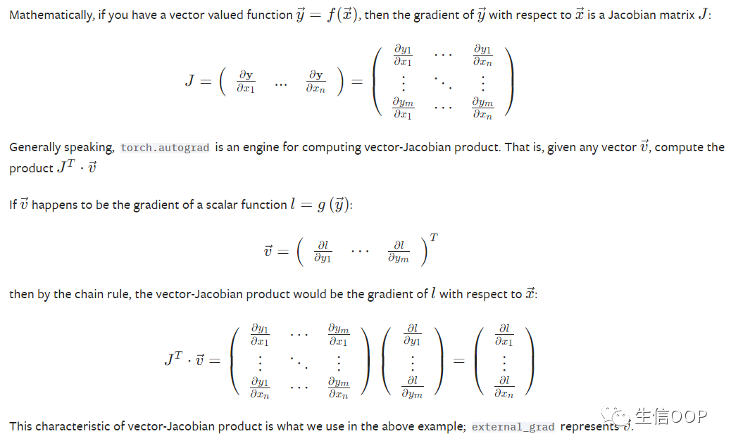
(留)4. Optional Reading - Vector Calculus using autograd
5. Computational Graph
Conceptually, autograd keeps a record of data (tensors) & all executed operations (along with the resulting new tensors) in a directed acyclic graph (DAG) consisting of Function objects. In this DAG, leaves are the input tensors, roots are the output tensors. By tracing this graph from roots to leaves, you can automatically compute the gradients using the chain rule.

Below is a visual representation of the DAG in our example. In the graph, the arrows are in the direction of the forward pass. The nodes represent the backward functions of each operation in the forward pass. The leaf nodes in blue represent our leaf tensors a and b.
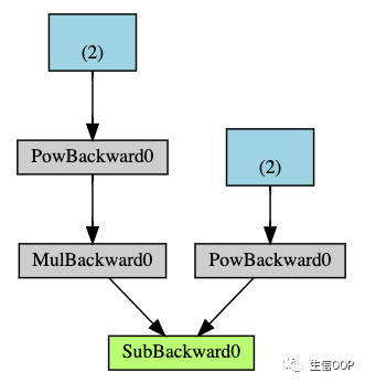
DAGs are dynamic in PyTorch,相当于在训练模型时,每迭代一次都会重新构建一个新的计算图。
6. Exclusion from the DAG
torch.autograd
tracks operations on all tensors which have their requires_grad
flag set to True
. For tensors that don’t require gradients, setting this attribute to False
excludes it from the gradient computation DAG.
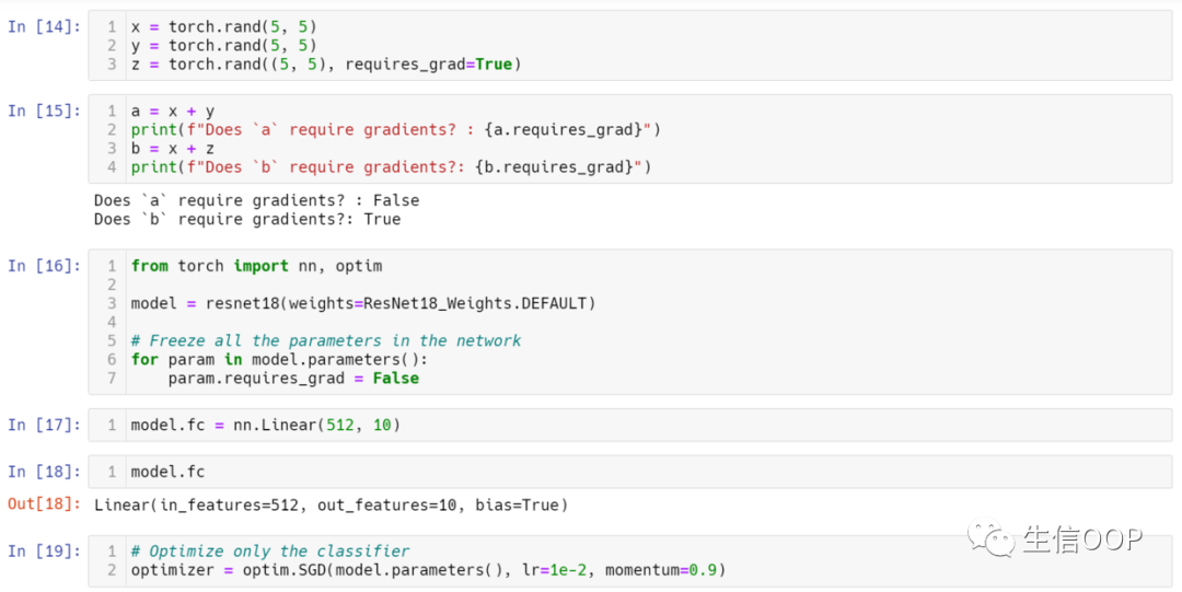
The output tensor of an operation will require gradients even if only a single input tensor has requires_grad=True
.
x = torch.rand(5, 5)
y = torch.rand(5, 5)
z = torch.rand((5, 5), requires_grad=True)
a = x + y
print(f"Does `a` require gradients? : {a.requires_grad}")
b = x + z
print(f"Does `b` require gradients?: {b.requires_grad}")复制
In a NN, parameters that don’t compute gradients are usually called frozen parameters. It is useful to “freeze” part of your model if you know in advance that you won’t need the gradients of those parameters (this offers some performance benefits by reducing autograd computations).
Another common usecase where exclusion from the DAG is important is for finetuning a pretrained network. In finetuning, we freeze most of the model and typically only modify the classifier layers to make predictions on new labels. (模型的微调)
from torch import nn, optim
model = resnet18(weights=ResNet18_Weights.DEFAULT)
# Freeze all the parameters in the network
for param in model.parameters():
param.requires_grad = False复制
Let’s say we want to finetune the model on a new dataset with 10 labels. In resnet, the classifier is the last linear layer model.fc
. We can simply replace it with a new linear layer (unfrozen by default) that acts as our classifier.
Now all parameters in the model, except the parameters of model.fc, are frozen. The only parameters that compute gradients are the weights and bias of model.fc
.
预训练模型最终是1000个labels,此处替换成10个labels,即改最后的一个input为512,output为1000的线性层,变为(512, 10),除此层外,其他参数处于“冻结”状态,不再计算参数梯度,即微调(finetune)。
model.fc = nn.Linear(512, 10)
# Optimize only the classifier
optimizer = optim.SGD(model.parameters(), lr=1e-2, momentum=0.9)复制
Notice although we register all the parameters in the optimizer, the only parameters that are computing gradients (and hence updated in gradient descent) are the weights and bias of the classifier.
The same exclusionary functionality is available as a context manager in torch.no_grad()
.
(留)Further readings:
In-place operations & Multithreaded Autograd
Example implementation of reverse-mode autodiff
参考:
https://pytorch.org/tutorials/beginner/blitz/autograd_tutorial.html https://www.youtube.com/watch?v=tIeHLnjs5U8 https://blog.csdn.net/PolarisRisingWar/article/details/116069338 https://towardsdatascience.com/machine-learning-for-beginners-an-introduction-to-neural-networks-d49f22d238f9 https://juejin.cn/post/6844903934876729351
