Oracle数据库如何选择创建什么样的直方图？

介绍

我经常被问及“Oracle如何知道在哪个列上需要直方图？”，以及，“为什么我会在我的主键列上得到一个直方图？”。Jonathan Lewis在不久前回应第二个问题时，贴出过一个解释点此查看。但我觉得最好在这个主题上说得多一些，并且聚焦在Oracle如何选择哪个列上应该有直方图上。特别是我想澄清，如果你使用建议（默认）的方法收集统计信息，即DBMS_STATS.GATHER…STATS的参数METHOD_OPT被设置为“FOR ALL COLUMNS SIZE AUTO”时，数据库如何决定创建什么直方图。

Oracle数据库可以创建多种类型的直方图（混合，TOP频率，频率），我将在后面简要介绍它们。但是，本文的目的不是详细讨论它们之间的差异，我想集中于导致直方图创建的一般情况。

本文针对Oracle Database 12c Release 1及以后的版本

你可能已经知道直方图对于改善基数评估十分有用，特别是列上的数据是倾斜时。如你所了解的，这不是故事的全部，我将从倾斜（skew）的含义开始说起。

倾斜（skew）是什么

数据库认为有两类倾斜。而对于我们大多数人来说，脑海中只有一种类型。下面是一张表示某宠物店售出的每种鱼有多少订单的示意图：

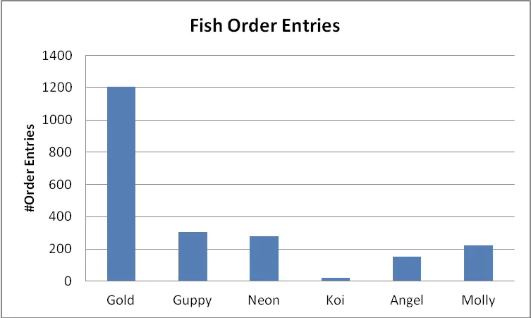
该店有很多金鱼的订单；它们便宜且普通。另一方面，锦鲤的价值高，价格也昂贵，所以，并不奇怪其售出得很少。从技术上讲，在值的重复度上存在不平均，或者说值倾斜。换句话说，部分鱼的名字明显比其它更经常出现。让我们来看两个简单的查询：

select sum(order_amount) from fish_sales where fish = 'Gold';    [1200 rows match]
select sum(order_amount) from fish_sales where fish = 'Koi';     [22 rows match]

对于上面的查询，匹配WHERE子句的行数是显著不同的，所以为优化器提供一种方法解决这个问题是有用的。这就是直方图的作用。

还有另外一类倾斜，我将用几个示例来展示它。

例 1
想像一个小型的，但快速成长的公司，其总是在雇佣新员工。员工信息存储在STAFF表中，该表包含有一个HIRE_DATE列。回到公司初创时期，通常要经历数周才会有一位新员工，但随着入职率的提高，对于任意给定日，我们可以绘制出类似下面的雇佣人数图：

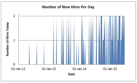
使用类似如下的查询，生成了上面的图：

select trunc(hire_date) "Date"
      ,count(*)         "Number of Hires Today"
from staff
group by trunc(hire_date)
order by trunc(hire_date);

你可以看到，在2012年的大部分日期没有雇佣，但是在2015年，几乎每一天都有多人加入。对于给定的雇佣日期范围，数据库在STAFF表中匹配的行数上有大范围的变化。从技术上讲，在范围上存在不平均，或者说范围倾斜。为了说清楚我的意思，考虑下面的查询：

select avg(salary) from staff where hire_date 
   between to_date('01-mar-2012') and to_date('30-apr-2012');

select avg(salary) from staff where hire_date 
   between to_date('01-mar-2014') and to_date('30-apr-2014');

尽管两个查询的范围大小是相同的（由于2012年是闰年，所以，我很小心的避免包括2月），第一个查询会匹配到少量的行，而第二个会匹配到大量的行。如果一个查询在HIRE_DATE的给定范围上过滤出的行数，预期会在匹配行数上看到大范围的变化，我们要帮助优化器识别出来的话。我们将需要一个直方图。

在本例中，还存在值倾斜。我提及该事实，是因为我想指出范围和值倾斜并不是互斥的：列值有时会在不同程度上，表现出这两种类型的倾斜。

例 2
可能最简单的方法看到范围倾斜，就是像下面这样包含唯一数值的列:

1, 100, 200, 300, 301, 302, 303, 304,…, 998, 999, 1000

每一个值只出现一次，但是出现在范围1到100的值的数量，与出现在范围300到400,和400到500是完全不同的。这类似于前面提到的Jonathan的示例是类似的。

例 3

当我们考虑数值或日期列时，很容易想像在缺失的值或日期上出现范围倾斜。而对于基于字符的字段，就不是那么直观了。就我个人经验，我喜欢将范围倾斜想像为我们使用一个固定的范围，并且在数据集上上下滑动，会有多少行匹配范围谓词。考虑下面的例子（真实的）：一张包含有美国姓氏清单的表，范围倾斜很容易像下面这样暴露出来：

select count(*) from us_surnames where surname between 'A' and 'C';      [19281 rows]
select count(*) from us_surnames where surname between 'H' and 'J';      [9635 rows]
select count(*) from us_surnames where surname between 'X' and 'Z';      [1020 rows]

例 4
最后，并不总是像例3中显示的那样明显，考虑下面的数据集：

AA, AB, AC, AD,…,AZ, BA, BB, BC,…, ZX, ZY, ZZ

它并不是像看起来那样没有任何间隔。但请记住，是有非字母字符的，并且我们可以在范围谓词中使用更长或更短的字符串。以下两个查询均返回0行：

select count(*)
from   the_table
where  column_value between 'B1' and 'B9';


select count(*) 
from   the_table
where  column_value between 'AZB' and 'B';

直方图会产生更好的基数评估，因为它使优化器可以感知到这些间隔。当使用范围查询谓词时，数据库编码列值并使用统计技术来描述基数评估方面的变化程度。一旦这个分析完成，由内部的阈值来决定直方图是否有用。

最终的结果，如果基于文本的列被用于范围查询谓词，那通常会生成直方图。

自动直方图创建

当收集统计信息时，METHOD_OPT使用的是SKEWONLY和AUTO选项，直方图是自动创建的。例如：

EXEC DBMS_STATS.GATHER_TABLE_STATS( … METHOD_OPT=>'FOR ALL COLUMNS SIZE SKEWONLY' …)

如果你选择使用“FOR ALL COLUMNS SKEWONLY”，那么所有列（不包括类似LONG和LOB数据类型的列）都需要测试来看一看是否需要直方图。这不是日常统计信息收集的最佳选择，因为有一个更有效的选项（这也是默认选项时会发生的）：

EXEC DBMS_STATS.GATHER_TABLE_STATS( … METHOD_OPT=>'FOR ALL COLUMNS SIZE AUTO' …)

AUTO使用“列使用信息”来识别哪些列被用在查询谓词和连接谓词中，使它们成为直方图的候选者。当统计信息被收集时，候选列被测试以进一步识别倾斜并计算列上唯一值数量。在许多情况下，将这些测试限制在最初的候选列名单上，会使AUTO比SKEWONLY更有效率。

对于这篇文章的其余部分，你可以假设使用了“For ALL COLUMNS SIZE AUTO”。此外，请记住，某些列数据类型不适用于直方图（如LONG和CLOB）。

列使用情况

Oracle数据库如何知道一个特定的列是在查询谓词或连接谓词中使用的呢？这个信息是由优化器在解析时收集，并最终存储在名为SYS.COL_USAGE$的Oracle数据字典表中。

我们可以使用DBMS_STATS应用接口，来得到用户友好的列使用情况数据的视图。在下面的例子中，该报告告诉我们STAFF表中的HIRE_DATE列被用于了范围谓词：

set long 10000
select dbms_stats.report_col_usage(user, 'staff') from dual;


DBMS_STATS.REPORT_COL_USAGE(USER,'STAFF')
--------------------------------------------------------------------------------
LEGEND:
.......
EQ         : Used in single table EQuality predicate
RANGE      : Used in single table RANGE predicate
LIKE       : Used in single table LIKE predicate
NULL       : Used in single table is (not) NULL predicate
EQ_JOIN    : Used in EQuality JOIN predicate
NONEQ_JOIN : Used in NON EQuality JOIN predicate
FILTER     : Used in single table FILTER predicate
JOIN       : Used in JOIN predicate
GROUP_BY   : Used in GROUP BY expression
...............................................................................
###############################################################################
COLUMN USAGE REPORT FOR ADHOC.STAFF
...................................
1. HIRE_DATE                           : RANGE
###############################################################################

如果你要自己测试这一功能，则要注意列使用情况数据，是周期性地刷新到数据字典的，所以，如果你正使用测试脚本，那么你可能并不能立即看到数据。如果你急于看到，你可以启动类似下面的手动刷新：

execute dbms_stats.flush_database_monitoring_info()

识别候选列

我们已经知道，数据库有一种方法确定哪个列被用在查询中。如果列用于连接或查询谓词，则它被视为直方图的候选列。例如，以下的这些查询会让col1和txtcol列成为潜在的直方图候选列：

Query:                                                                  Column usage:

select sum(amount) from sales where col1 = 10;                          [EQ]
select sum(amount) from sales where col1 != 10;                         [recorded as EQ]
select sum(amount) from sales where col1 > 10;                          [RANGE]
select sum(amount) from sales s, customers c where s.col1 =  c.col1;    [EQ_JOIN]
select sum(amount) from sales s, customers c where s.col1 != c.col1;    [EQ_JOIN NONEQ_JOIN]
select sum(amount) from sales where txtcol like 'ALA%';                 [LIKE]

一旦列使用情况信息被用于了识别候选列，数据库需要检测这些列上的数据，来确定对于改善基数评估，直方图是否是有用的。这发生在统计信息被收集时（比如使用DBMS_STATS.GATHER_TABLE_STATS时），但数据库使用什么原则来最终决定它? 我下面接着说。

有用的直方图

数据库采用一些原则来决定一个直方图是否是有用的。直方图将被视为是有用的，如果满足：

1. 列存在值倾斜，并且列使用情况显示其用于 RANGE, LIKE, EQ 或 EQ_JOIN.
2. 列存在范围倾斜，并且列使用情况显示其用于 LIKE 或 RANGE.
3. 列具有少量的唯一值（有一些重复值），并且列使用情况显示其用于 RANGE, LIKE, EQ or EQ_JOIN.
4. 当增量统计信息被使用, 且甚至分区中的列上并不存在值倾斜或范围倾斜，直方图也有可能被创建。数据库要使用分区级的直方图去推导出全局直方图。为非倾斜列创建的直方图，会被优化器统计信息忽略。

你会看到原则1和原则3是有重叠的，而且，在原则3中，没有提及倾斜。其原因是Oracle认为对于少量唯一值（NDV)的列，直方图是有用的，即使没有明显的范围或值倾斜（假设有一些重复值）。这样做的一个典型好处是，在值和范围两方面，数据分布都是十分平均，但仍然存在“空洞”值的情况下，在低基数列上创建直方图的成本是低的，因此，如果列被用于连接或谓词中，只有很少的理由不去创建它。在实践中，这意味着使用RANGE、LIKE、EQ或EQ_JOIN列并且NDV小于或等于254的列将被给予频率直方图（如果NDV略高于254，甚至是TOP频率直方图）。

值254是重要的，因为这是默认的直方图桶数，并且这是考虑选择使用何种直方图时的其中一个因素。更多信息请点击这里.

还有一些额外的复杂内容我没有涉及。比如，直方图可能是从部分或全部采样的数据（取决于如何和何时统计信息被收集）中创建的。数据类型是重要的点。比如，如果你在数值列上使用LIKE谓词，那么这类的使用信息不会被记录到列使用情况中。“倾斜”和“非倾斜”的边界是一个统计结构（或者，你喜欢的话，可以看做是一个模糊结构），且列值可以既是范围倾斜，也是值倾斜的。不管怎样，我希望你现在能理解其工作的一般原则了。

欢迎评论。

原文链接：https://blogs.oracle.com/optimizer/post/how-does-the-oracle-database-choose-what-histograms-to-create

How does the Oracle Database choose what histograms to create?
June 10, 2019 | 8 minute read
Nigel Bayliss
Product Manager

Introduction

I am often asked, “How does Oracle choose which columns need a histogram?” Also, “Why have I got a histogram on my primary key column?” Jonathan Lewis posted an explanation in response to the latter question some while ago, but I thought I’d cover a little bit more on this topic and focus on how Oracle chooses which columns should have histograms. In particular, I want to clarify how the database determines what histograms to create if you use the recommended (default) method for gathering statistics, which is where the DBMS_STATS.GATHER…STATS parameter METHOD_OPT is set to ’FOR ALL COLUMNS SIZE AUTO’.

The Oracle Database can create a variety of different types of histogram (hybrid, top frequency, frequency) and I will mention them briefly below. However, for the purposes of this post it is not necessary to dwell on the differences between them. I want instead to concentrate on the circumstances that lead to histogram creation in general.

This post is aimed at Oracle Database 12c Release 1 onwards.

You will probably know already that histograms are useful for improving cardinality estimates, particularly if the data in a column is skewed. As you will see, this is not the full story, but I will start by covering what is meant by skew.

What is Skew?

There are two types of skew considered by the database. For most of us, there is one type that springs to mind. Here is a chart representing how many order entries a pet shop has for each type of fish it sells:

The shop gets a lot of orders for goldfish; they are cheap and common. On the other hand, Koi carp are highly valued and expensive so it’s not surprising that fewer are sold. Technically speaking, there is a non-uniformity in the repetitions of values or value skew. In other words, some fish names appear significantly more often than others. Let’s take a look at a couple of simple queries:

select sum(order_amount) from fish_sales where fish = 'Gold';    [1200 rows match]
select sum(order_amount) from fish_sales where fish = 'Koi';     [22 rows match]

For the above queries, the number of rows matching the WHERE clause are very different so it would be useful to give the optimizer a way to figure this out. That is what a histogram is for of course.

There is another type of skew, and I will illustrate it with a few examples.

Example 1

Imagine a small but fast-growing company that is hiring new people over time. Employee information is stored in a STAFF table, which includes a HIRE_DATE column. Back in the days when the company started up it was common for a number of weeks to pass between each new hire, but gradually the rate of arrival increased. For any given day we can plot the number of people hired like this:

I generated the plot above using a query like this:

select trunc(hire_date) "Date"
      ,count(*)         "Number of Hires Today"
from staff
group by trunc(hire_date)
order by trunc(hire_date);

You will see that a large number of days passed in 2012 with no hires, but in 2015 there were multiple people joining almost every day. There is a wide variation in the number of rows the database will match in the STAFF table for a given range of hire dates. Technically speaking, there is a non-uniformity in range or range skew. To clarify what I mean, consider the following queries:

select avg(salary) from staff where hire_date 
   between to_date('01-mar-2012') and to_date('30-apr-2012');

select avg(salary) from staff where hire_date 
   between to_date('01-mar-2014') and to_date('30-apr-2014');

The first query will match a small number of rows and the second will match a large number of rows even though the size of the range is the same in both cases (I was careful to avoid including February since 2012 is a leap year!). We need to help the optimizer figure out that if a query filters rows over a given range of HIRE_DATE values, then it can expect to see a wide variation in the number of rows it will match. We are going to need a histogram.

There is value skew in this example too. I mention this fact because I want to point out that range and value skews are not mutually exclusive: column values can sometimes exhibit both types of skew to varying degrees.

Example 2

Perhaps the simplest way to see range skew is to consider a column containing unique numeric values like this:

1, 100, 200, 300, 301, 302, 303, 304,…, 998, 999, 1000

Each value happens only once but the numbers of values falling into the range of (1,100) is very different from those falling into range of (300, 400) and (400, 500). This is similar to Jonathan’s example mentioned above.

Example 3

When considering numeric or date columns, it is easy to visualize range skew in terms of missing values or days. For character-based fields it is not so intuitive. Personally, I like to think of range skew in terms of how many rows will match a range predicate if we take a fixed range and 'slide it up and down’ the dataset. Consider the following (real) example: a table containing a list of US surnames. Range skew is easily revealed like this:

select count(*) from us_surnames where surname between 'A' and 'C';      [19281 rows]
select count(*) from us_surnames where surname between 'H' and 'J';      [9635 rows]
select count(*) from us_surnames where surname between 'X' and 'Z';      [1020 rows]

Example 4

Finally, it is not always quite as obvious as example 3 implies. Consider a dataset like this:

AA, AB, AC, AD,…,AZ, BA, BB, BC,…, ZX, ZY, ZZ

It doesn’t look like there are any gaps at all, but remember that there are non-alphabet characters and we could use longer and shorter strings in the range predicates. Both of the following queries return a count of zero:

select count(*)
from   the_table
where  column_value between 'B1' and 'B9';


select count(*) 
from   the_table
where  column_value between 'AZB' and 'B';

A histogram will yield better cardinality estimates because it will make the optimizer aware of these gaps. The database encodes column values and uses statistical techniques to characterize the degree of variation in cardinality estimates when a range-based query predicate is used. Once this analysis is complete, internal thresholds are used to decide whether or not a histogram will be useful.

The net result is that text-based columns will often acquire histograms if they are used in range-based query predicates.

Automatic Histogram Creation

Histograms are created automatically when statistics are gathered using the SKEWONLY and AUTO options in METHOD_OPT. For example:

EXEC DBMS_STATS.GATHER_TABLE_STATS( … METHOD_OPT=>'FOR ALL COLUMNS SIZE SKEWONLY' …)

If you choose to use FOR ALL COLUMNS SKEWONLY, then all columns will need to be tested to see if they require a histogram (excluding columns with datatypes such as LONG and CLOB). This is not the best choice for day-to-day statistics collection because there is a more efficient option (which also happens to be the default):

EXEC DBMS_STATS.GATHER_TABLE_STATS( … METHOD_OPT=>'FOR ALL COLUMNS SIZE AUTO' …)

AUTO uses column usage information to identify which columns are used in query predicates and joins, making them potential candidates for a histogram. When statistics are gathered, the candidate columns are tested further to identify skew and calculate the number of distinct column values. Restricting these tests to an initial list of candidates will, in many cases, make AUTO much more efficient than SKEWONLY.

For the remainder of this post you can assume that ‘FOR ALL COLUMNS SIZE AUTO’ is used. In addition, remember that some column datatypes are not eligible for histograms (such as LONG and CLOB).

Column Usage

How does the Oracle Database know that a particular column is used in a query predicate or join? This information is gathered by the Oracle Optimizer at parse time and ultimately stored in the Oracle data dictionary in a table called SYS.COL_USAGE$.

We can get a user-friendly view of column usage data using the DBMS_STATS API. In the following example, the report tells us that the HIRE_DATE column in STAFF was used in a range predicate:

set long 10000
select dbms_stats.report_col_usage(user, 'staff') from dual;


DBMS_STATS.REPORT_COL_USAGE(USER,'STAFF')
--------------------------------------------------------------------------------
LEGEND:
.......
EQ         : Used in single table EQuality predicate
RANGE      : Used in single table RANGE predicate
LIKE       : Used in single table LIKE predicate
NULL       : Used in single table is (not) NULL predicate
EQ_JOIN    : Used in EQuality JOIN predicate
NONEQ_JOIN : Used in NON EQuality JOIN predicate
FILTER     : Used in single table FILTER predicate
JOIN       : Used in JOIN predicate
GROUP_BY   : Used in GROUP BY expression
...............................................................................
###############################################################################
COLUMN USAGE REPORT FOR ADHOC.STAFF
...................................
1. HIRE_DATE                           : RANGE
###############################################################################

If you want to test this for yourself, then note that column usage data is flushed to the data dictionary periodically, so if you are using a test script then you might not see the data immediately. If you are in a hurry, you can initiate a manual flush like this:

execute dbms_stats.flush_database_monitoring_info()

Identifying Candidate Columns

We have established that the database has a way of determining how individual columns are used in queries. A column is considered a candidate for a histogram if it is used in joins or query predicates. For example, the following queries will make col1 and txtcol potential candidates for histograms:

Query:                                                                  Column usage:

select sum(amount) from sales where col1 = 10;                          [EQ]
select sum(amount) from sales where col1 != 10;                         [recorded as EQ]
select sum(amount) from sales where col1 > 10;                          [RANGE]
select sum(amount) from sales s, customers c where s.col1 =  c.col1;    [EQ_JOIN]
select sum(amount) from sales s, customers c where s.col1 != c.col1;    [EQ_JOIN NONEQ_JOIN]
select sum(amount) from sales where txtcol like 'ALA%';                 [LIKE]

Once column usage information has been used to identify candidate columns, the database needs to examine the data in those columns to establish whether a histogram will be useful for improving cardinality estimates. This happens when statistics are gathered (e.g. when using DBMS_STATS.GATHER_TABLE_STATS), but what principles does the database use to finally decide? I will cover that next.

Beneficial Histograms

The database applies some principles to decide whether a histogram will be of benefit. A histogram will be deemed beneficial if:

1. The column has value skew and column usage indicates RANGE, LIKE, EQ or EQ_JOIN.
2. The column has range skew and column usage indicates LIKE or RANGE.
3. The column has a low number of distinct values (with some repeated values) and column usage indicates RANGE, LIKE, EQ or EQ_JOIN.
4. When incremental statistics are used, and even though a column might not have value/range skew in a partition, a histogram may be created. The database will use partition-level histograms to derive global histograms. Histograms created for non-skewed data are ignored by optimizer stats.

You will see that there is overlap between principles 1 and 3, and there is no mention of skew in number 3. The reason is that Oracle considers histograms useful for low number of distinct value (NDV) columns even if there is no significant range or value skew (provided that there are some repeated values). A typical benefit of doing this is in the case where a data distribution is quite uniform in both value and range but there are nevertheless some “holes” in values. The cost of building histograms on low cardinality columns is small, so if a column is used in joins or predicates then there is little reason not to create one. In practice this means that a column with usage RANGE, LIKE, EQ or EQ_JOIN columns and an NDV of less than or equal to 254 will be given a frequency histogram (or even a top frequency histogram if the NDV is a little over 254).

The number 254 is significant because it is the default histogram bucket count and is one of the factors taken into account when choosing the type of histogram used. There is more on this here.

There is some additional complexity I have not covered. For example, histograms may be created from a partial or full sample of the data (depending on how and when statistics are gathered). Datatypes can be important. For example, if you use a LIKE predicate on a numeric column, then this type of usage will not be recorded in column usage. The boundary between “skewed” and “non-skewed” is a statistical construct (or, if you prefer, a “fuzzy” construct) and column values can have both range skew and value skew. Nevertheless, I hope that you now appreciate the general principles at work.

Comments welcome.