


我最近在帮助客户升级一个大的数据仓库时,遇到了这个问题。升级前,当他们在他们的大表上收集统计信息时,使用了值为0.000001的ESTIMATE_PERCENT,这是允许的最小采样值。当我询问为何选择了如此小的采集大小时,他们说这是因为他们在每天加载数据后,需要在分区和全局级,以特别快的速度收集统计信息。
由于这些大表是分区的,我认为增量统计信息会是他们的一个优选方案。但是,为了使用增量统计信息收集,你必须让ESTIMATE_PERCENT的参数值为默认的AUTO_SAMPLE_SIZE。 尽管客户了解使用增量统计信息的好处,但他们不想修改ESTIMATE_PERCENT的值。所以我表示,使用AUTO_SAMPLE_SIZE,他们得到的统计信息等效于100%采样的效果,但却是采样10%的速度。由于我们会采用增量统计信息,仅需要在新加载数据的分区上收集统计信息,而全局统计信息(表级统计信息)会自动正确的聚合。
所以,他们抱着极大的怀疑,在测试系统中尝试了增量统计信息,并惊喜于其所花费的时间。然而,他们不相信所收集的统计信息,并问我“我要如何比较使用AUTO_SAMPLE_SIZE得到的统计信集和使用值为0.000001的ESTIMATE_PERCENT所得到的统计信息?”
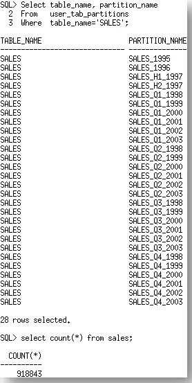
回答它很容易,“使用DBMS_STAT.DIFF_TABLE_STATS”。 尽管说起来很容易,但帮助他们找到如何正确的使用 DBMS_STAT.DIFF_STATS 函数的过程,却是不简单的。在本文中,我希望分享一些你在使用DIFF_STATS时,可能会遇到的不太明显的陷阱。让我们使用SH用户下的SALES表做为例子。SALES表上有28个分区及918843行。
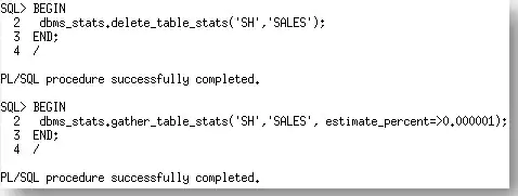
首先,我们将使用他们初始的设置ESTIMATE_PERCENT为0.000001来收集SALES表上的统计信息。
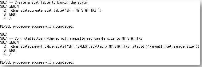
这些统计信息现在可以备份到一个新创建的统计信息表。
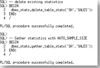
现在我们有了一个来自于手动指定ESTIMATE_PERCENT运行的统计信息的导出。让我们使用默认值AUTO_SAMPLE_SIZE,在SALES表上再次收集。
现在,我们准备使用 DBMS_STAT.DIFF_TABLE_STATS函数来比较SALES表上的两个统计信息集合。根据被比较的统计信息所在的位置,该函数实际上有三个版本
- DBMS_STAT.DIFF_TABLE_STATS_IN_HISTORY
- DBMS_STAT.DIFF_TABLE_STATS_IN_PENDING
- DBMS_STAT.DIFF_TABLE_STATS_IN_STATTAB
在本例中,我们会使用DBMS_STAT.DIFF_TABLE_STATS_IN_STATTAB函数。该函数还会比较依赖对象(索引,列,分区)的统计信息,并只显示那些统计信息的差异超过特定阈值(%)的对象的统计信息。该阈值也可以做为函数的参数来指定;默认值是10%。第一个来源的相关统计信息会被做为计算百分比差异的基础
DBMS_STAT.DIFF_TABLE_STATS函数是表函数,所以,当你使用SELECT时,需要使用关键字table,否则,你会收到一个错误,提示对象不存在。

表函数返回一个报告和最大差异的百分比(数值)。为了正确显示,你需要使用set long命令定义LONG的宽度,以便报告可以恰当的显示。

现在,我们知道了如何生成报告,让我们看看它说了什么。
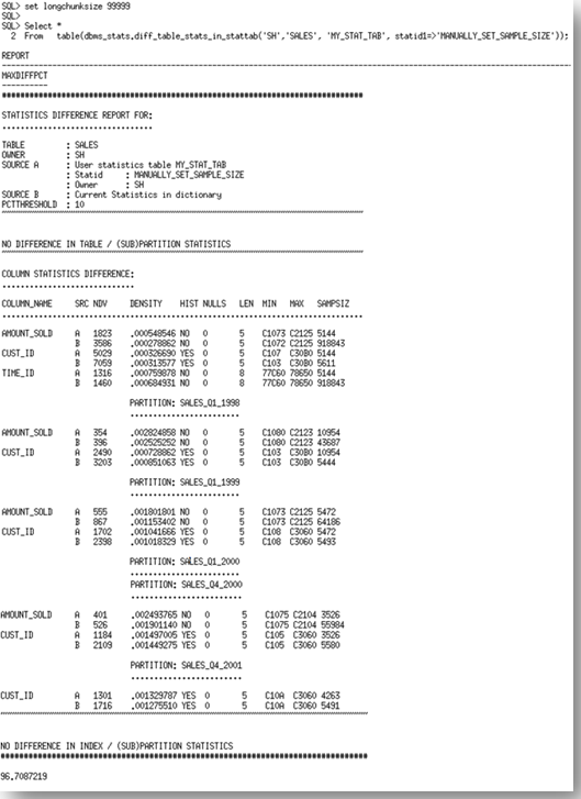
报告有三个部分。它以基表统计信息的比较来开始。在本例中,表的统计信息(行数,块数等)是相同的。由于我们可以从一个非常小的采样,准确推测出表的统计信息,所以,目前为止的结果是预料中的。报告的第二部分检查列上的统计信息。
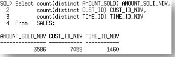
列出了统计信息不同的每一个列,以及每一个来源的统计信息值。来源A是STATTAB,来源B是数据字典中的当前统计信息,在我们的示例中是AUTO_SAMPLE_SIZE的集合。你会注意到统计信息中一个非常明显的不同,尤其是在每个列上的NDV(不同值的数量)和最小最大值。如果我们比较这些结果和实际的不同值的数量(如下),我们看到由来源B,即AUTO_SAMPLE_SIZE的统计信息是更准确的。
报告继续列出每一个分区中列统计信息不同的。在这个部分,你会看到问题只发生在AMOUNT_SOLD,CUST_ID列上。SALES表是在TIME_ID列上的范围分区,所以,在每个分区中的TIME_ID是有限的,因此在这个级别上两个结果之间差异的百分比不足以满足10%的阈值。
报告的最后查看索引统计信息。在本例中,索引统计信息是不同的,但是并没有超过10%的不同,所以,报告中没有显示。
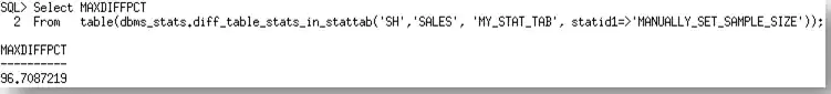
随报告一起返回的还有最大差异百分比,这是统计信息之间差异的最大百分比。这些差异可以来自于表,列或者索引的统计信息。在本例中,最大差异百分比是96%!
所以,使用AUTO_SAMPLE_SIZE的统计信息是明显不一样的。而且事实胜于雄辩,我们将新的统计信息用于测试环境,发现优化器基于新统计信息选择了更好的执行计划。好到他们可以将大量之前因糟糕的统计信息而在他们代码中使用的HINT删除掉。你不能要求比这更好的了。
你可以获得我用来生成本文的脚本的拷贝,点这里。
原文链接:https://blogs.oracle.com/optimizer/post/how-do-i-compare-optimizer-statistics
How Do I Compare Optimizer Statistics?
January 31, 2020 | 6 minute read
Maria Colgan
Distinguished Product Manager
This question came up recently when I was helping a customer upgrade a large data warehouse. Prior to the upgrade, they were using an ESTIMATE_PERCENT of 0.000001, the smallest possible sample size allowed, when they gathering statistics on their larger tables. When I asked why they picked such a tiny sample size they said it was because they needed statistics to be gathered extremely quickly after their daily load both at the partition and at the global level.
Since these large tables were partitioned, I thought they would be an excellent candidate for incremental statistics. However, in order to use incremental statistics gathering you have to let the ESTIMATE_PERCENT parameter default to AUTO_SAMPLE_SIZE. Although the customer saw the benefit of using incremental statistics they were not keen on changing the value of ESTIMATE_PERCENT. So I argued that with AUTO_SAMPLE_SIZE they would get statistics that were equivalent to a 100% sample but with the speed of a 10% sample. Since we would be using incremental statistics we would only have to gather statistics on the freshly loaded partition and the global statistics (table level statistics) would be automatically aggregated correctly.
So with much skepticism, they tried incremental statistics in their test system and they were pleasantly surprised at the elapse time. However, they didn’t trust the statistics that were gathered and asked me, “how do I compare the statistics I got with AUTO_SAMPLE_SIZE to the statistics I normally get with an ESTIMATE_PERCENT of 0.000001?”
The answer to that was easy, ‘use DBMS_STAT.DIFF_TABLE_STATS’. Although the answer was easy, it wasn’t an easy process to help them to work out how to use the DBMS_STAT.DIFF_STATS functions correctly. In this post I hope to share some of the gotchas you many encounter using DIFF_STATS that are not so obvious. Let’s take the SALES table from the SH schema as an example. The SALES table has 28 partitions and 918843 rows.
First we will gather statistics on the SALES table with their original setting for ESTIMATE_PERCENT, 0.00001.
These statistics can now be backed up into a newly created stats table.
Now that we have an export of the statistics from the manually specified ESTIMATE_PERCENT run, let’s re-gather statistics on the SALES table using the default, AUTO_SAMPLE_SIZE.
So, we are now ready to compare the two sets of the statistics for the SALES table using the DBMS_STAT.DIFF_TABLE_STATS function. There are actually three version of this function depending on where the statistics being compared are located;
- DBMS_STAT.DIFF_TABLE_STATS_IN_HISTORY
- DBMS_STAT.DIFF_TABLE_STATS_IN_PENDING
- DBMS_STAT.DIFF_TABLE_STATS_IN_STATTAB
In this case we will be using the DBMS_STAT.DIFF_TABLE_STATS_IN_STATTAB function. The functions also compare the statistics of the dependent objects (indexes, columns, partitions) and will only displays statistics for the object(s) from both sources if the difference between the statistics exceeds a certain threshold (%). The threshold can be specified as an argument to the function; the default value is 10%. The statistics corresponding to the first source will be used as the basis for computing the differential percentage.
The DBMS_STAT.DIFF_TABLE_STATS functions are table functions so you must use the key word table when you are selecting from them, otherwise you will receive an error saying the object does not exist.
The table function returns a report (clob datatype) and maxdiffpct (number). In order to display the report correctly you must use the set long command to define the width of a long so the report can be displayed properly.
How that we know how to generate the report, let’s look at what it says,
The report has three sections. It begins with a comparison of the basic table statistics. In this case the table statistics (number of rows, number of blocks etc) are the same. The results so far are to be expected since we can accurately extrapolate the table statistics from a very small sample. The second section of the report examines column statistics.
Each of the columns where the statistics vary is listed (AMOUNT_SOLD, CUST_ID, TIME_ID) along with a copy of the statistics values from each source. Source A is the STATTAB, which in our case is the ESTIMATE_PERCENT of 0.000001. Source B is the statistics currently in the dictionary, which in our case is the AUTO_SAMPLE_SIZE set. You will notice quite a significant difference in the statistics, especially in the NDV (number of distinct values) and the minimum and maximum values for each of the columns. If we compare these results with the actual number of distinct values for these (below), we see that the statistics reported by source B, the AUTO_SAMPLE_SIZE are the most accurate.
The report then goes on to list the column statistics differences for each of the partitions. In this section you will see that the problems occur only in the AMOUNT_SOLD, CUST_ID columns. The SALES table is range partitioned on TIME_ID, so there is a limited number of TIME_IDs in each partition, thus the percentage difference between the results on this level is not enough to meet the threshold of 10%.
Finally the report looks at the index statistics.In this case the index statistics were different but they were not greater than 10% different so the report doesn’t show them.
Along with the report the function returns the MAXDIFFPCT. This is the maximum percentage difference between the statistics. These differences can come from the table, column, or index statistics. In this case the MAXDIFFPCT was 96%!
So the statistics were significantly different with AUTO_SAMPLE_SIZE but the proof is in the pudding. We put the new statistics to the test and found that the Optimizer chose much better execution plan with the new statistics. So much so they were able to remove a ton of hints from their code that had been necessary previously due to poor statistics. You can’t ask for anything better than that!
You can get a copy of the script I used to generate this post here.
