R数据分析|标准化回归系数

本文主要介绍如何对R语言lm() 函数下的线性回归模型进行标准化，并获取其标准化回归系数，主要使用lm.beta package。回归系数及标准化回归系数如下图所示：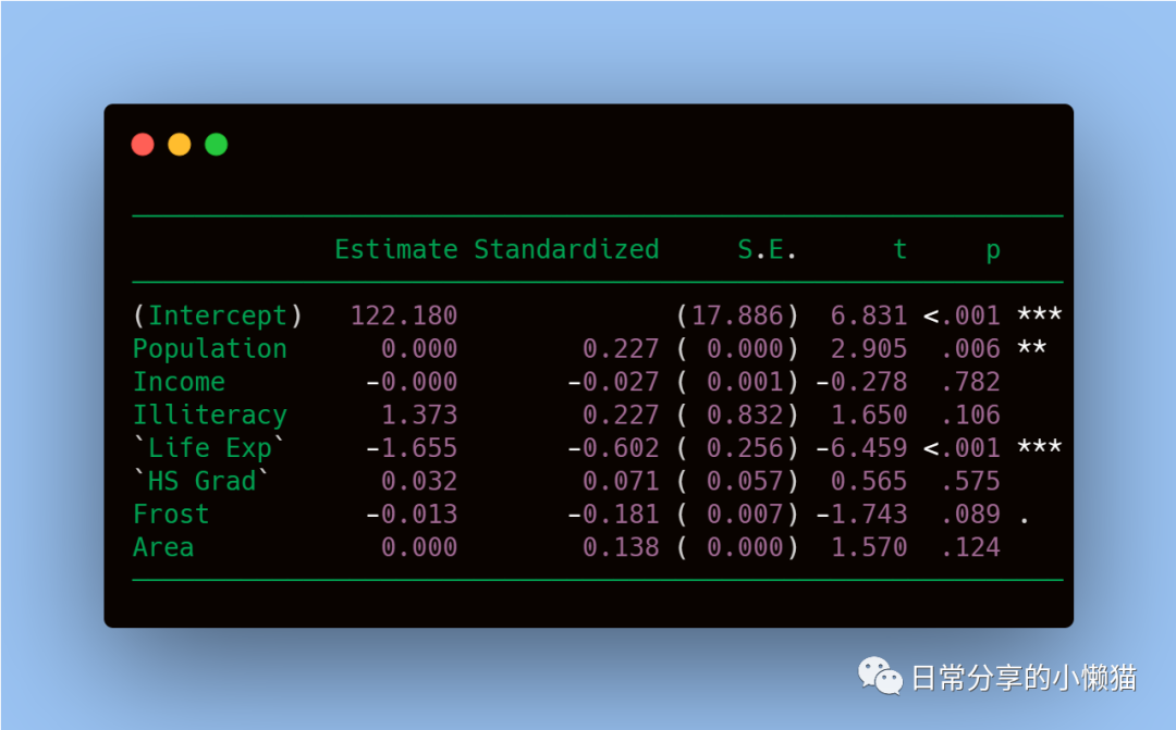

1、模型准备

使用R语言中自带的state.x77数据集，构建因变量为Murder
的线性回归模型。

install.packages("lm.beta")
library(tidyverse)
library(lm.beta)
states <- state.x77 %>% as.data.frame()
head(states)
#           Population Income Illiteracy Life Exp Murder HS Grad Frost   Area
#Alabama          3615   3624        2.1    69.05   15.1    41.3    20  50708
#Alaska            365   6315        1.5    69.31   11.3    66.7   152 566432
#Arizona          2212   4530        1.8    70.55    7.8    58.1    15 113417
#Arkansas         2110   3378        1.9    70.66   10.1    39.9    65  51945
#California      21198   5114        1.1    71.71   10.3    62.6    20 156361
#Colorado         2541   4884        0.7    72.06    6.8    63.9   166 103766

lm.model <- lm(Murder ~ ., data = states) #OLS
lm.model.std <- lm.beta(lm.model) #对回归模型进行标准化

2、模型对比

2.1 模型摘要

未标准化

summary(lm.model) #未标准化

标准化

summary(lm.beta(lm.model)) #标准化
summary(lm.model.std) #标准化

2.2 回归系数及标准误、t值、p值等

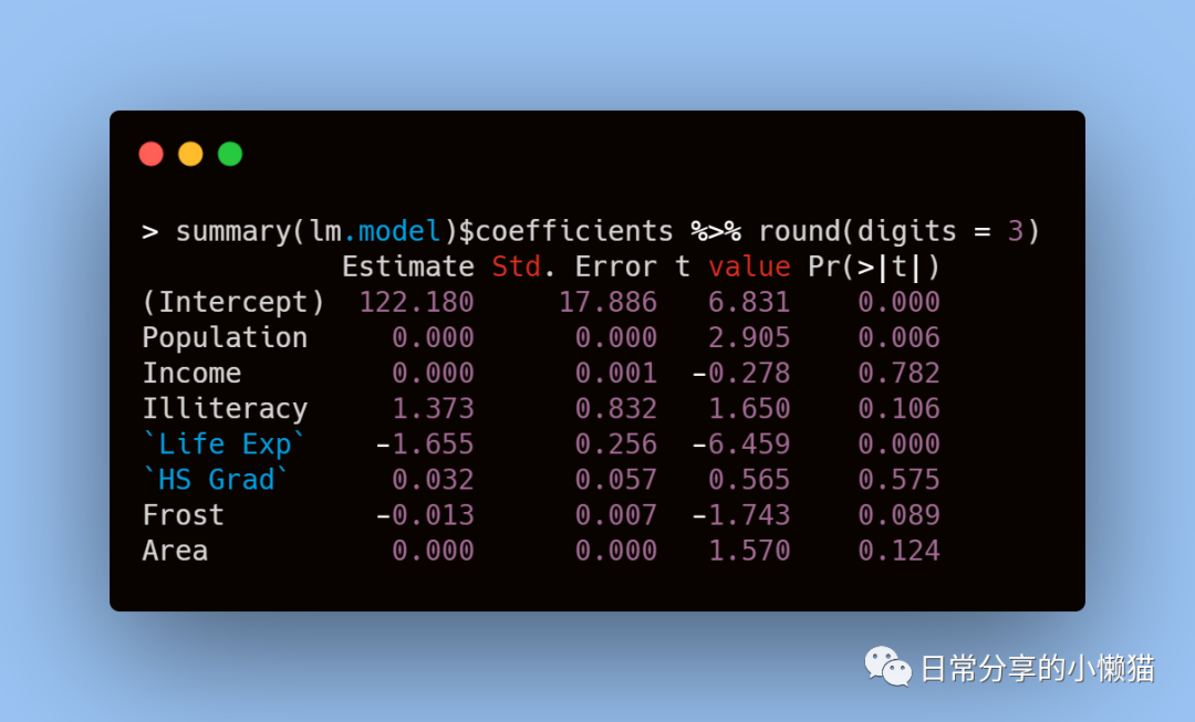
未标准化

summary(lm.model)$coefficients %>% round(digits = 3)

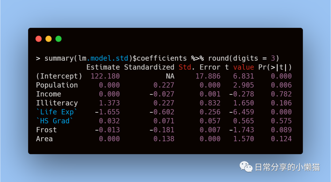
标准化

summary(lm.model.std)$coefficients %>% round(digits = 3)

2.3 95%置信区间

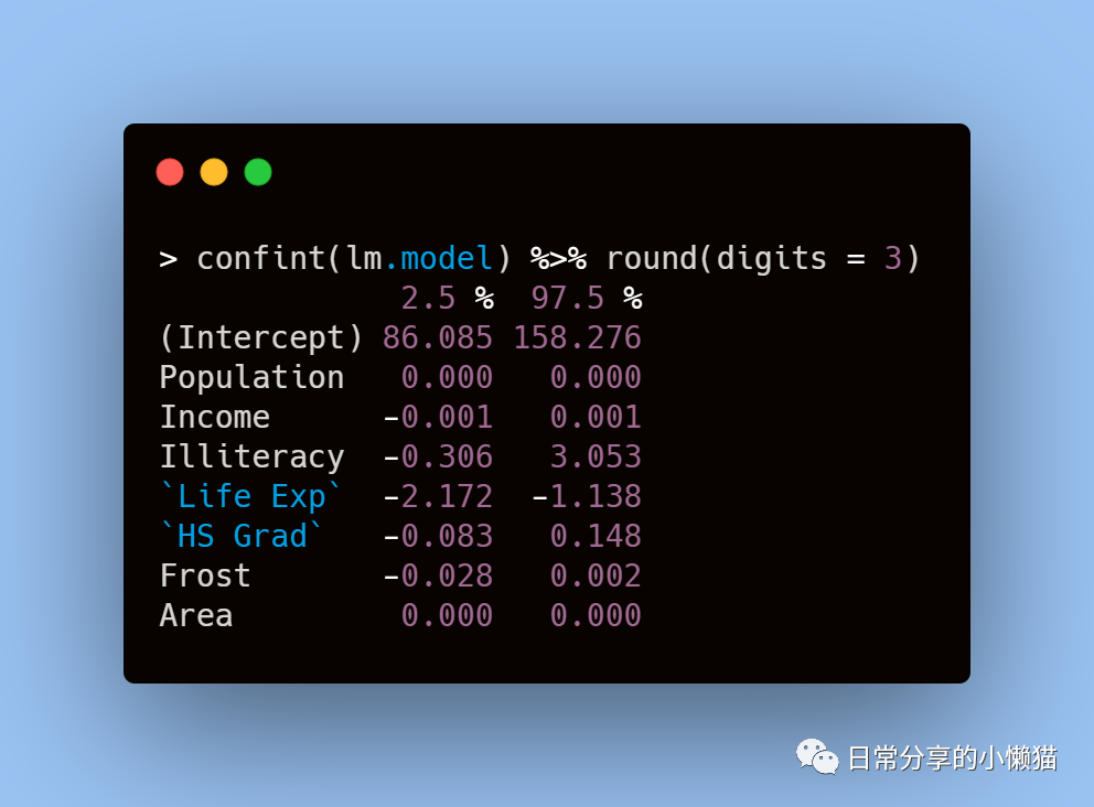
未标准化

confint(lm.model) %>% round(digits = 3)

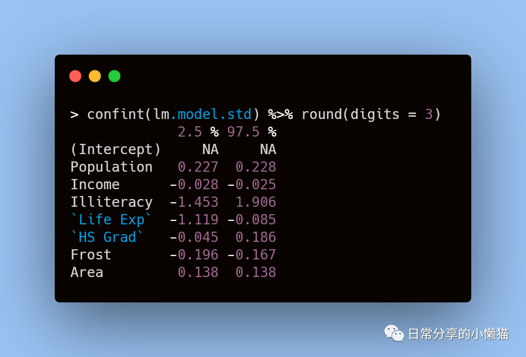
标准化

confint(lm.model.std) %>% round(digits = 3) 

3、回归系数可视化

利用coefplot包中的coefplot() 函数，可快速实现回归系数的可视化。

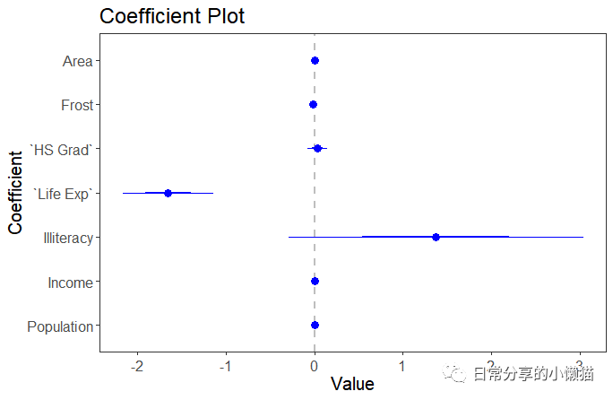
3.1 未标准化回归系数

install.packages("coefplot")
library(coefplot)
coefplot(lm.model, intercept = FALSE)

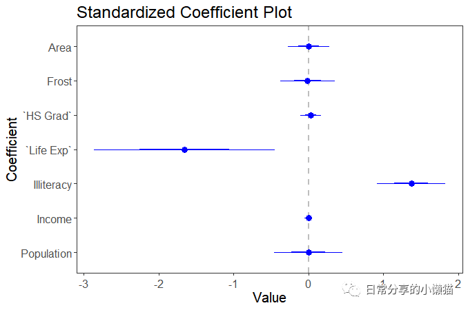
3.2 标准化回归系数

coefplot(lm.model.std, title = "Standardized Coefficient Plot")

4、其他

关于回归系数可视化可进一步阅读R语言绘图|回归系数可视化。其他绘图方法可进一步阅读公众号其他文章。

如有帮助请多多点赞哦！