


 |
前置准备
下附conda建立环境命令
conda create -n pygeo38 python=3.8 -y && conda activate pygeo38 && conda install -c conda-forge geopandas rasterio && python -m ipykernel install --user --name pygeo38 --display-name "GeoPython 3.8"
conda activate pygeo38
连续变量重分类——重庆市高程重分类
2.1 导入相关库
from pathlib import Path # 处理文件路径import rasterio as riofrom rasterio.plot import showimport numpy as npimport matplotlib.pyplot as plt
data_path = Path(r'.\data')dem_file = data_path "dem.tif"
with rio.open(dem_file) as f:
    nodata = f.nodata
    meta = f.meta
    data = f.read(1)
    data[data == nodata] = np.nan
    show(f, cmap='terrain')
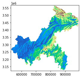
with rio.open(dem_file) as f:nodata = f.nodatameta = f.metadata = f.read(1)data[data == nodata] = np.nanshow(f, cmap='terrain')
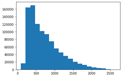
data_flat = data.flatten()plt.hist(data.flatten(), 20);
2.3 重分类断点构建
breaks = np.arange(300, 2401, 300)array([ 300, 600, 900, 1200, 1500, 1800, 2100, 2400])2.4 条件判断构建方法
简单条件判断
先做个小例子:
array1 = np.array([1, 2, 3, 4, 5])np.where(array1%2 == 0, array1*-1, array1**2)
array([ 1, -2, 9, -4, 25])嵌套条件判断
先做个小例子:
建立一个1到10的数组,当数值小于等于3,赋值为1,大于3小于等于8赋值为2, 大于8赋值为3。
array1 = np.arange(1, 11)np.where(array1 <= 3, 1,np.where(array1 <= 8, 2, 3))
array([1, 1, 1, 2, 2, 2, 2, 2, 3, 3])
2.5 栅格数据重分类
data_reclass = np.where(np.isnan(data), 0,np.where(data<300, 1,np.where(data<600, 2,np.where(data<900, 3,np.where(data<1200, 4,np.where(data<1500, 5,np.where(data<1800, 6,np.where(data<2100, 7,np.where(data<2400, 8, 9))))))))).astype(np.int8)
两种其他形式的写法
breaks = np.arange(300, 2401, 300) # 不包含最小值array_name = "data"data_reclass = eval(f"np.where(np.isnan({array_name}), np.nan, \n" + "\n".join([f"np.where({array_name} < {b}, {v}, " for v, b in enumerate(breaks, start=1)]) + f"{len(breaks)+1}" + ")" * (len(breaks)+1))
breaks = np.arange(0, 2401, 300) # 包含最小值data_reclass = np.sum(np.dstack([(data >= b) for b in breaks]), axis=2)
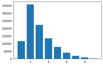
2.6 重分类结果一览
x_, y_ =np.unique(data_reclass, return_counts=True)plt.bar(x_[1:], y_[1:])f, axes = plt.subplots(1, 2, figsize=(20, 10))show(data, transform=meta["transform"], cmap='terrain', ax=axes[0])show(data_reclass, transform=meta["transform"], cmap='terrain', ax=axes[1])for ax in axes:ax.set_xticklabels([])ax.set_yticklabels([])plt.subplots_adjust(wspace=0, hspace=0)

文章转载自我得学城,如果涉嫌侵权,请发送邮件至:contact@modb.pro进行举报,并提供相关证据,一经查实,墨天轮将立刻删除相关内容。
