Selective Data Acquisition in the Wild for Model Charging.pdf

章芋文

492

13页

6次

2023-07-27

免费下载

Selective Data Acquisition in the Wild for Model Charging

Chengliang Chai

Tsinghua University

Beijing, China

ccl@mail.tsinghua.edu.cn

Jiabin Liu

Tsinghua University

Beijing, China

liujb19@mails.tsinghua.edu.cn

Nan Tang

QCRI

Doha, Qatar

ntang@hbku.edu.qa

Guoliang Li

Tsinghua University

Beijing, China

liguoliang@tsinghua.edu.cn

Yuyu Luo

Tsinghua University

Beijing, China

luoyy18@mails.tsinghua.edu.cn

ABSTRACT

The lack of sucient labeled data is a key bottleneck for practition-

ers in many real-world supervised machine learning (ML) tasks. In

this paper, we study a new problem, namely selective data acquisi-

tion in the wild for model charging: given a supervised ML task and

data in the wild (e.g., enterprise data warehouses, online data repos-

itories, data markets, and so on), the problem is to select labeled

data points from the data in the wild as additional train data that

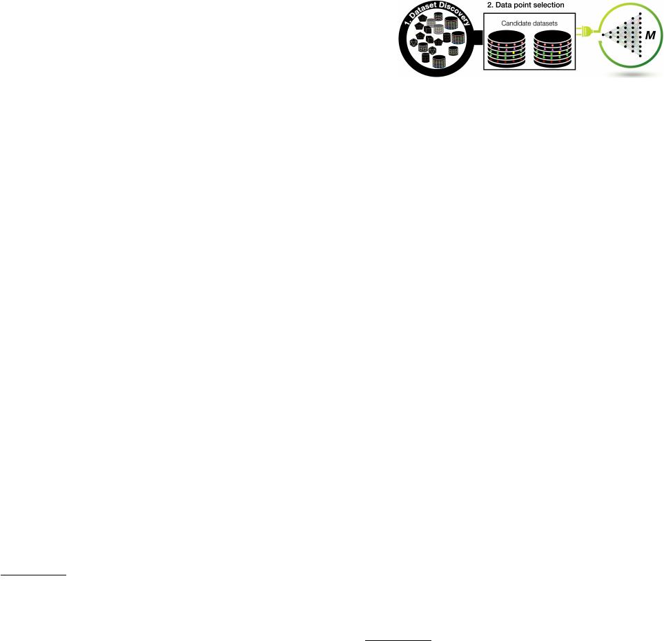
can help the ML task. It consists of two steps (Fig. 1). The rst step

is to discover relevant datasets (e.g., tables with similar relational

schema), which will result in a set of candidate datasets. Because

these candidate datasets come from dierent sources and may fol-

low dierent distributions, not all data points they contain can help.

The second step is to select which data points from these candidate

datasets should be used. We build an end-to-end solution. For step

1, we piggyback o-the-shelf data discovery tools. Technically, our

focus is on step 2, for which we propose a solution framework called

AutoData

. It rst clusters all data points from candidate datasets

such that each cluster contains similar data points from dierent

sources. It then iteratively picks which cluster to use, samples data

points (i.e., a mini-batch) from the picked cluster, evaluates the

mini-batch, and then revises the search criteria by learning from

the feedback (i.e., reward) based on the evaluation. We propose a

multi-armed bandit based solution and a Deep Q Networks-based

reinforcement learning solution. Experiments using both relational

and image datasets show the eectiveness of our solutions.

PVLDB Reference Format:

Chengliang Chai, Jiabin Liu, Nan Tang, Guoliang Li, and Yuyu Luo.

Selective Data Acquisition in the Wild for Model Charging. PVLDB, 15(7):

1466-1478, 2022.

doi:10.14778/3523210.3523223

1 INTRODUCTION

Data-centric ML. In many supervised ML projects, the main bot-

tleneck is the lack of sucient labeled train data (a.k.a. data-centric

This work is licensed under the Creative Commons BY-NC-ND 4.0 International

License. Visit https://creativecommons.org/licenses/by-nc-nd/4.0/ to view a copy of

this license. For any use beyond those covered by this license, obtain permission by

emailing info@vldb.org. Copyright is held by the owner/author(s). Publication rights

licensed to the VLDB Endowment.

Proceedings of the VLDB Endowment, Vol. 15, No. 7 ISSN 2150-8097.

doi:10.14778/3523210.3523223

Figure 1: Selective data acquisition for model charging.

ML) [

], not which ML models to use and how to op-

timize these models (a.k.a. model-centric ML), especially for ML

practitioners.

Example 1.

[

Insucient train data.

]

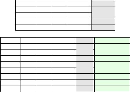
Consider Fig. 2(a) that shows

a dataset

𝑇

train

, which is used to train a regression model to predict

the house

Price

at Kolkata, India, based on the features (

City

Year

Area

Security

). The test data

𝑇

test

is given in Fig. 2(b), whose

Price

values are to be predicted. The ground truth

Price

values are

also provided for helping the discussion.

Figure 3(a) shows both the learned model using only

𝑇

train

(i.e.,

Line 1) and the ground truth model that we want to learn (i.e., Line 2).

Because

𝑇

train

is small and does not contain sucient data points

(e.g., there are many houses with

Area >

1000 or

700 in

𝑇

test

, but

all houses in

𝑇

train

have

Area

in the range

[

700

1000

]

), the mo del

trained using 𝑇

train

(i.e., Line 1) is not good enough for 𝑇

test

Data acquisition. The process of getting more labeled data is

known as data acquisition, which is categorized into two classes:

human-in-the-loop and automatic data acquisition. Human-in-the-

loop data acquisition includes weak supervision where users need to

dene rules (e.g., Snorkel [

], data programming [

]), and crowd-

and expert-sourcing. Automatic data acquisition uses automatic

methods to obtain more train data.

Selective data acquisition in the wild for model charging. We

ask whether it is possible to nd useful data points from the data in

the wild as shown in Fig. 1 so as to “charge” the model, where we

know that dierent datasets may follow dierent data distributions,

but meanwhile, we also hypothesize that some data points can help.

For doing so, the rst step is to select candidate datasets. For

tables, this is known as data discovery with many o-the-shelf

The rst two authors contributed equally to this research. Guoliang Li is the corre-

sponding author.

City Year Area Security Price

Kolkata 2009 710 No 3,200,000

Kolkata 2013 770 No 3,850,000

Kolkata 2007 935 No 2,524,000

Kolkata 2006 973 Yes 3,611,000

(a) 𝑇

train

: Train dataset (learn to predict “Price”).

City Year Area Security Price Ground Truth

Kolkata 2017 350 No ? 2,100,000

Kolkata 2019 465 Yes ? 4,365,000

Kolkata 2015 572 No ? 3,268,000

Kolkata 2012 655 Yes ? 2,599,000

Kolkata 2012 735 No ? 3,300,000

Kolkata 2017 881 Yes ? 4,698,000

Kolkata 2011 1123 Yes ? 3,324,000

Kolkata 2014 1210 Yes ? 5,000,000

(b) 𝑇

test

: Test dataset (predict the “Price” column).

Figure 2: Sample train and test datasets.

tools [

]. For images, there are many benchmarks, as well

as Web APIs such as Google, Baidu or Azure image search.

Example 2.

[

Using all data points in candidate datasets.

]

Fig. 3(b)(c) and (d) show three datasets that also contain house price

information in dierent cities of India, i.e.,

𝐷

and

𝐷

for Ban-

glore, Mumbai, and Delhi, respectively. They have dierent schemata

with 𝑇

train

and 𝑇

test

in Fig. 2, but they can be used as train data.

A straightforward solution is to add all these datasets to the train

data (i.e.,

𝑇

train

= 𝑇

train

∪ 𝐷

) and train a model. By

doing so, we can obtain a model as shown in Fig. 3(a) Line 3, which,

unfortunately, deviates far from the ground truth model Line 2.

Our question is that: given candidate datasets, whether selecting

some data points will be better than using all?

Example 3.

[

Selected data points.

]

If we can select “good” data

points, such as

{𝑟

}

from

𝐷

{𝑠

, 𝑠

}

from

𝐷

, and

{𝑡

, 𝑡

}

from

𝐷

as additional train data that are highlighted in Figs. 3(b–d), we

can use them in Fig. 3(a) (i.e., those annotated by green frames) and

train a model Line 4. Clearly, Line 4 is much closer, thus better than

Line 1 and Line 3, to the ground truth model Line 2.

Example 1 shows that more labeled data is needed. Example 2

tells us using all data points is not ideal. Example 3 shows it is more

benecial to select some data points.

Challenges. There are two essential challenges. First, candidate

datasets may come from various data distributions that are dierent

from the desired data distribution of the ML task, which is unknown.

Second, many data points in these candidate sets are not good w.r.t.

our ML task, which raises the challenge that how can we eectively

select and measure which new data points should be added.

Contributions. Our contributions are summarized as follows.

(1) Selective data acquisition in the wild for model charging.

We study the problem of automatic data acquisition for supervised

ML in a new setting where the supervised ML task does not have

enough train data, and it has access to the data in the wild (Section 2).

Note that datasets in the wild are heterogeneous and not all of data

points can help the task.

(2) A solution framework. We propose a solution framework (see

Fig. 1) that consists of two steps: dataset discovery that selects

candidate datasets and data points selection that selects data

points from these candidate datasets. (Section 3)

(3)

AutoData

with multi-arme d bandit. We introduce a classi-

cal multi-armed bandit based solution to handle the exploration-

exploitation trade-o for AutoData. (Section 4)

(4)

AutoData

with Deep Q Network-based reinforcement learn-

ing (RL). Another eective model is to use Deep Q learning based

RL, which learns a neural network to approximate the Q-table (i.e., a

simple but huge lookup table that calculates the maximum expected

future rewards for action at each state) that decides which cluster

to select based on the current status. (Section 5)

(5) Evaluation. We conduct extensive experiment to show that

our methods can eectively select data points from dierent data

sources and improve the ML performance by maximum 14.8% and

8.3% on relational and image datasets, respectively. (Section 6)

2 PRELIMINARY

Supervise d machine learning. We consider supervised ML as

training a model

𝑀

to learn a function

𝑓 ()

that maps an input to

an output based on example input-output pairs as 𝑓 : X → Y.

We use

𝑀 (𝐴)

to denote the model

𝑀

that is trained with dataset

𝐴

, and the notation

𝑀 (𝐴, 𝐵)

to denote the model

𝑀

that is trained

with 𝐴 and is evaluated with dataset 𝐵.

Train/validation/test datasets. A set of labeled dataset

𝑇

typically split into three disjoint subsets as train/validation/test

(𝑇

train

/𝑇

val

/𝑇

test

). 𝑇

test

is completely held-out during training.

Data in the wild. We use the term data in the wild to generally

refer to all datasets that one can have access to, including data lakes,

data markets, online data repositories, enterprise data warehouses,

and so on. More specically, for supervised ML, we consider it as a

set of datasets

D = {𝐷

, . . . , 𝐷

𝑚

}

, where

𝐷

𝑖

(

𝑖 ∈ [

,𝑚]

) is a set of

(data point, label) pairs.

Candidate datasets. The candidate datasets w.r.t. a supervised ML

task

𝑀

, denoted by

𝑐

, is a subset of

that contains datasets

“relevant” to

𝑀

. For tabular data, the relevance typically means that

these candidate datasets have the same or highly overlapping rela-

tional schema with

𝑇

train

. For image data, the relevance typically

means that these candidate datasets contain images that have the

same labels (e.g., {cat, dog, bird, sh}) as 𝑇

train

Candidate data pool. The candidate data pool (or simply data

pool), denoted by

, is the union of all data points in the candidate

datasets, i.e., P =

(𝑥,𝑦) ∈𝐷

𝑖

,𝐷

𝑖

∈D

𝑐

(𝑥, 𝑦).

Selective data acquisition for model charging. Given a super-

vised ML task with a pre-specied model

𝑀

, train/validation/test

datasets (

𝑇

train

𝑇

val

𝑇

test

), and a candidate data pool

, the prob-

lem is to select a subset

∗

⊂ P

using

𝑇

train

and

𝑇

val

, such that

it can obtain the most performance improvement of the super-

vised ML task on

𝑇

test

∗

= arg max

′

⊂ P

𝑀 (𝑇

train

∪P

′

,𝑇

test

) −

𝑀 (𝑇

train

,𝑇

test

Example 4.

[

Selective data acquisition.

]

Given an ML task of

training a regression model using

𝑇

train

as shown in Fig. 2 and a data

of 13

免费下载

关注

评论