ZTE-Predictor Disk Failure Prediction System Based on LSTM.pdf

章芋文

111

4页

4次

2023-08-29

免费下载

ZTE-Predictor: Disk Failure Prediction System Based on LSTM

Hongzhang Yang

†‡

, Zongzhao Li

‡

, Huiyuan Qiang

‡

, Zhongliang Li

‡

, Yaofeng Tu

‡

, and Yahui Yang

†*

†

School of Software & Microelectronics, Peking University, China

‡

ZTE Corporation, China

Corrsponding Author: yhyang@ss.pku.edu.cn

Abstract—Disk failure prediction technology has become a

hotspot in both academia and industry, which is of great

significance to improve the reliability of data center. This

paper studies ZTE's disk SMART (Self-Monitoring Analysis

and Reporting Technology) data set, trying to predict whether

the disk will fail within 5-7 days. In the model training stage,

the disk

state is classified as normal and failure within 5 days

Then the positive and negative samples are balanced by both

over-sampling and under-sampling. Finally, the data set is

trained by LSTM (Long Short-Term Memory) and the disk

failure prediction model is obtained. In the experiment of ZTE

historical data set, the best FDR (Fault Detection Rate) is 97.4%

and FAR (False A

larm

Rate) is 0.3%. After launching in ZTE

data center for 7 months, the best FDR is 94.5%, and the FAR

is 0.7%.

Keywords—Disk; Failure; LSTM; Prediction

I. INTRODUCTION AND MOTIVATION

With the advent of the era of big data, digital data has

become precious. Most of the world's data is stored in disks.

Massive data storage makes the stability of disks face great

challenges. Once a disk is failed, the data stored in it may be

lost forever. Although the disk can be backed up redundantly,

it will increase the cost, and data loss will still occur when

multiple disks are damaged. According to Backblaze’s report

[1] in 2019, the annual failure rate of disk is 1.25%, making

maintenance extremely difficult [2]

. In a ZTE data center

with 25,000 disks, disks fail almost every day.

Disk failures are generally dived into unpredictable

failures and predictable failures. Unpredictable failures are

often caused by unexpected accidents, which will not be

discussed in this paper. For predictable failures, the

abnormal external vibration, the abnormal temperature and

humidity around the disk, and the increase of read-write error

rate provide the possibility for the disk failure prediction.

Migration of the data ahead can greatly reduce the loss. Disk

failure prediction technology has become a hotspot in both

academia and industry, which is of great significance to

improve the reliability of data center.

In the related research [3]-[12], the main method is to

establish a status classification model based on the disk

status data, and then classify the disk data to be tested

according to the classification model. One type is normal and

the other is near-failure. The main constraint of this method

is the limited applicability. This is because the operation and

maintenance personnel can only know that the

disk

is about

to fail, but how long it will fail is unknown, and it is difficult

to grasp the timing of disk replacement. Changing disks too

early causes a lot of disk life cycles to be wasted. Changing

disks too late can easily lead to permanent irreparable data.

Based on ZTE's needs for efficient disk management, we

consider that it is reasonable to predict disk failures about 5-

7days in advance.

This paper studies the SMART [13] dataset collected by

ZTE once a day, trying to predict whether the disk will fail

within 5-7 days. The disk status is classified as normal or

failure within 5 days. After that, the positive and negative

samples are balanced by over sampling and under sampling.

Finally, the characteristic data is trained and the disk failure

prediction model is obtained. In the experimental stage,

based on the ZTE historical data set, this paper compares

different data balance methods, different sample_days,

different training rounds, different algorithm effects, and

carries out targeted optimization in data center for 7 months,

and achieves good results.

II. P

REDICTOR DESIGN AND IMPLEMENTATION

Because data of different disk brands have some

attributes that are different, the research object of this paper

is a total of 73,

942 Seagate disks in ZTE's data center,

including 3,119 failure disks within 2 years.

A. Sample label

SMART dataset is a set of attributes and sets threshold

values beyond which attributes should not pass under normal

operation. SMART is widely used for disk failure prediction.

Firstly, the change of SMART attribute of the disk before

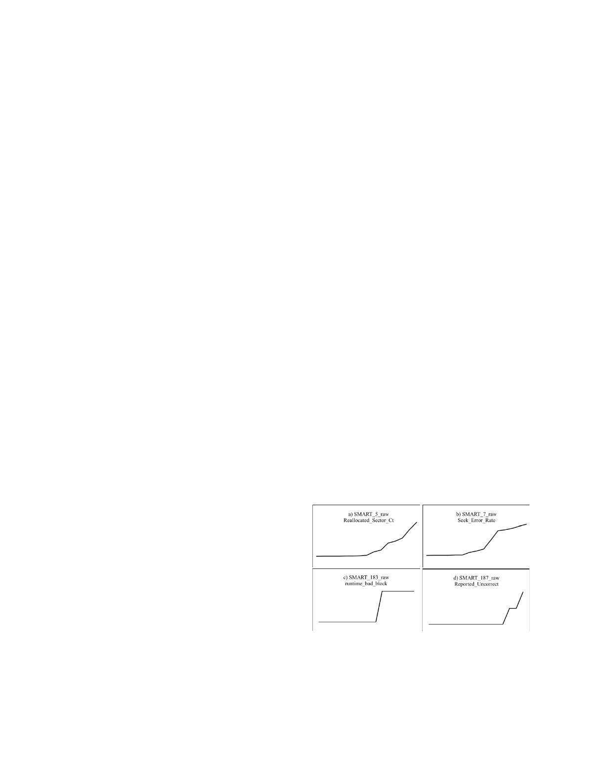
failure is observed. As is shown in

Figure 1

, the values of

SMART_5_raw, SMART_7_raw, SMART_183_raw, and

SMART_187_raw in the dataset before the failure changes

significantly, which are the most significant attributes for

prediction in this paper. Similar conclusions can be drawn

from the Backblaze dataset. We observe the status of a large

number of

disk

s and take into account the actual application

requirements, finally the disk is defined as the failed disk on

the 5th day before the failure.

Fig. 1. THE SUDDEN CHANGE OF FOUR SMART ATTRIBUTES BEFORE DISK

FAILURE

The original positive samples of the training set are

SMART attribute data of all failure disks within 5 days of the

failure

time, and the original negative samples of the training

set are SMART attribute data randomly selected 10 times

from every healthy disk. Therefore, there were 18,714

positive samples and 708,230 negative samples.

2020 50th Annual IEEE/IFIP International Conference on Dependable Systems and Networks - Supplemental Volume (DSN-S)

DOI 10.1109/DSN-S50200.2020.00017

Authorized licensed use limited to: ZTE CORPORATION. Downloaded on August 29,2023 at 01:53:42 UTC from IEEE Xplore. Restrictions apply.

B. Feature engineering

Due to occasional SMART acquisition failures or errors

in transmitting data sets, missing value padding is necessary.

The method we adopted in this paper is: if the missing values

are consecutive 2 or more, then the mode of the SMART

item on the disk is used as the filling value; if there is only

one missing value

, the average of the value before and after

it is used as the filling value.

Data normalization uses the interval scaling method,

which uses Max and Min in a feature to scale all values to

the interval of [0, 1].

Sample_days and predict_failure_days are 2 important

parameters:

x Sample_days is defined as the time window size of

the input data of the LSTM network in each

sequence sample, for example,

sample_days

is 5, and

then a training sample will contain SMART attribute

information of the disk in the past 5 days. The

sample_days need to have appropriate values. If it is

too small, the potential information provided to the

LSTM is less. If it is too large, it corresponds to a

long time series. The data that is too far away from

the final failure has a small impact on the prediction

of the final failure tr

end, and may even be

misleading.

x Predict_failure_days is defined as the number of

days before the failure, which is an alarm boundary.

The value of predict_failure_days also needs to be

appropriate. Too long or too short a time interval

will affect the effectiveness of disk failure

processing. The value of predict_failure_days is

reasonable for 5-7 days.

Regarding feature selection, because deep learning

models automatically learn features and the feature

dimensions of the dataset involved 45 dimensions, of which

only 21 dimensions remain after filtering out features with

variance 0. There is no further feature selection in this paperˈ

so the selected features include: SMART_1_raw,

SMART_4_raw, SMART_5_raw, SMART_7_raw,

SMART_9_raw, SMART_12_raw, SMART_183_raw,

SMART_184_raw, SMART_187_raw, SMART_188_raw,

SMART_189_raw, SMART_190_raw, SMART_192_raw,

SMART_193_raw, SMART_194_raw, SMART_197_raw,

SMART_198_raw, SMART_199_raw, SMART_240_raw,

SMART_241_raw,and SMART_242_raw.

C. Dataset balancing

As other hard disk SMART datasets face the same

problem, the number of positive samples in ZTE datasets is

far less than the number of negative samples, which makes it

difficult for machine learning algorithm to obtain sufficient

positive sample information when training the model, so

FDR is relatively low, and it is necessary to balance the data.

This paper attempts four methods of sample balancing,

including ADASYN [14], SMOTE [15], ADASYN

combined with ENN [16], and SMOTE combined with ENN,

in order to compare the different prediction results. After

data balance, the number of positive and negative samples is

both 50,000. In the evaluation section, we will compare the

influence of data balance on the prediction effect.

D. Training model

Every disk goes through a process from health to failure,

so the SMART data collected periodically at a fixed time

period is time series. As a common algorithm, the memory of

the RNN model is generally within 7 time periods, and the

data entered early will gradually fail due to the disappearance

of the gradient. If only the SMART attribute is used to

change the time window of 7 days or less, it is far from

reflecting the change of the disk state. Fortunately, LSTM is

an improved version of RNN, which works better on

problems with time series characteristics. It stores memory

through the information conveyor, which solves the problem

of disappearance of gradient, so that this paper can use a

larger time window to disk prediction. In addition, for

comparison, this paper also tried common algorithms,

including RNN [10], AdaBoost [7], random forest [5], LOG

[5], SVM [5],

and decision tree [

5].

TABLE I. LSTM MODEL PARAMETER

Layer(type)

Output shape

lstm_1(LSTM)

(None, 30, 32)

lstm_2(LSTM)

(None, 30, 64)

lstm_3(LSTM)

(None, 128)

dense_1(Dense)

(None, 128)

dense_2(Dense)

(None, 64)

dense_3(Dense)

(None, 1)

As shown in Table 1, this paper uses the LSTM N to 1

model. The input is the data in the sample_days, and the

output is whether the failure will occur in 5 days. The output

is 1 if a failure

is about to occur, otherwise it is 0.

Considering the complexity of disk failure prediction rules,

this paper builds a neural network composed of 3 layers of

LSTM and 3 layers of Dense. The output dimensions of the

first 5 layers are 32, 64, 128, 128, 64, and the output

dimensions of the 6th layer are1.

III. E

VALUATIONS

In this chapter, firstly, training and testing are carried out

based on ZTE historical data set, and all samples are divided

into training set data and test set according to the proportion

of 8:2. During the test, different data balance methods,

different sample_days sizes, different training rounds, and

different algorithms are compared respectively. Each sample

is classified of failure or health. Then, within 7 months of

launch in ZTE data center, we predict whether there will be

any failure in the next 5-7 days based on each disk. In this

chapter, FDR and FAR are used as evaluation indexes.

A. Evaluations on historical data set

In this chapter, based on unbalancing, ADASYN,

SMOTE, ADASYN combined with ENN, and SMOTE

combined with ENN, the original dataset is preprocessed to

compare. In order to improve the efficiency, the number of

training iterations is limited to 50 rounds, and the

sample_days is set to 30. The experimental results are shown

in Table 2. Under the same factors of feature, model, and

predict_failure_days, compared with the unbalancing, the

over-

sampling method improves the FDR significantly, and

the combination of over-sampling and under-sampling

method reduces the FAR, further improving the prediction

effect. Among them, the best performance is SMOTE

combined with ENN, FDR is 89.2%, FAR is 9.3%, so this

method is used for data balance in subsequent experiments.

Authorized licensed use limited to: ZTE CORPORATION. Downloaded on August 29,2023 at 01:53:42 UTC from IEEE Xplore. Restrictions apply.

of 4

免费下载

关注

评论