1409.3215Sequence to Sequence Learning.pdf

nirvana

9页

0次

2023-11-20

5墨值下载

arXiv:1409.3215v3 [cs.CL] 14 Dec 2014

Sequence to Sequence Learning

with Neural Networks

Ilya Sutskever

Google

ilyasu@google.com

Oriol Vinyals

Google

vinyals@google.com

Quoc V. Le

Google

qvl@google.com

Abstract

Deep Neural Networks (DNNs) are powerful models that have achieved excel-

lent performance on difﬁcult learning tasks. Although DNNs work well whenever

large labeled training sets are available, they cannot be used to map sequences to

sequences. In this paper, we present a general end-to-end approach to sequence

learning that makes minimal assumptions on the sequence structure. Our method

uses a multilayered Long Short-Term Memory (LSTM) to map the input sequence

to a vector of a ﬁxed dimensionality, and then another deep LSTM to decode the

target sequence from the vector. Our main result is that on an English to French

translation task from the WMT’14 dataset, the translations produced by the LSTM

achieve a BLEU score of 34.8 on the entire test set, where the LSTM’s BLEU

score was penalized on out-of-vocabulary words. Additionally, the LSTM did not

have difﬁculty on long sentences. For comparison, a phrase-based SMT system

achieves a BLEU score of 33.3 on the same dataset. When we used the LSTM

to rerank the 1000 hypotheses produced by the aforementioned SMT system, its

BLEU score increases to 36.5, which is close to the previous best result on this

task. The LSTM also learned sensible phrase and sentence representations that

are sensitive to word order and are relatively invariant to the active and the pas-

sive voice. Finally, we found that reversing the order of the words in all source

sentences (but not target sentences) improved the LSTM’s performance markedly,

because doing so introduced many short term dependencies between the source

and the target sentence which made the optimization problem easier.

1 Introduction

Deep Neural Networks (DNNs) are extremely powerful machine learning models that achieve ex-

cellent performance on difﬁcult problems such as speech recognition [13, 7] and visual object recog-

nition [19, 6, 21, 20]. DNNs are powerful because they can perform arbitrary parallel computation

for a modest number of steps. A surprising example of the power of DNNs is their ability to sort

N N-bit numbers using only 2 hidden layers of quadratic size [27]. So, while neural networks are

related to conventional statistical models, they learn an intricate computation. Furthermore, large

DNNs can be trained with supervised backpropagation whenever the labeled training set has enough

information to specify the network’s parameters. Thus, if there exists a parameter setting of a large

DNN that achieves good results (for example, because humans can solve the task very rapidly),

supervised backpropagation will ﬁnd these parameters and solve the problem.

Despite their ﬂexibility and power, DNNs can only be applied to problems whose inputs and targets

can be sensibly encoded with vectors of ﬁxed dimensionality. It is a signiﬁcant limitation, since

many important problems are best expressed with sequences whose lengths are not known a-priori.

For example, speech recognition and machine translation are sequential problems. Likewise, ques-

tion answering can also be seen as mapping a sequence of words representing the question to a

sequence of words representing the answer. It is therefore clear that a domain-independent method

that learns to map sequences to sequences would be useful.

Sequences pose a challenge for DNNs because they require that the dimensionality of the inputs and

outputs is known and ﬁxed. In this paper, we show that a straightforward application of the Long

Short-Term Memory (LSTM) architecture [16] can solve general sequence to sequence problems.

The idea is to use one LSTM to read the input sequence, one timestep at a time, to obtain large ﬁxed-

dimensional vector representation, and then to use another LSTM to extract the output sequence

from that vector (ﬁg. 1). The second LSTM is essentially a recurrent neural network language model

[28, 23, 30] except that it is conditioned on the input sequence. The LSTM’s ability to successfully

learn on data with long range temporal dependencies makes it a natural choice for this application

due to the considerable time lag between the inputs and their corresponding outputs (ﬁg. 1).

There have been a number of related attempts to address the general sequence to sequence learning

problem with neural networks. Our approach is closely related to Kalchbrenner and Blunsom [18]

who were the ﬁrst to map the entire input sentence to vector, and is related to Cho et al. [5] although

the latter was used only for rescoring hypotheses produced by a phrase-based system. Graves [10]

introduced a novel differentiable attention mechanism that allows neural networks to focus on dif-

ferent parts of their input, and an elegant variant of this idea was successfully applied to machine

translation by Bahdanau et al. [2]. The Connectionist Sequence Classiﬁcation is another popular

technique for mapping sequences to sequences with neural networks, but it assumes a monotonic

alignment between the inputs and the outputs [11].

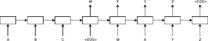
Figure 1: Our model reads an input sentence “ABC” and produces “WXYZ” as the output sentence. The

model stops making predictions after outputting the end-of-sentence token. Note that the LSTM reads the

input sentence in reverse, because doing so introduces many short term dependencies in the data that make the

optimization problem much easier.

The main result of this work is the following. On the WMT’14 English to French translation task,

we obtained a BLEU score of 34.81 by directly extracting translations from an ensemble of 5 deep

LSTMs (with 384M parameters and 8,000 dimensional state each) using a simple left-to-right beam-

search decoder. This is by far the best result achieved by direct translation with large neural net-

works. For comparison, the BLEU score of an SMT baseline on this dataset is 33.30 [29]. The 34.81

BLEU score was achieved by an LSTM with a vocabulary of 80k words, so the score was penalized

whenever the reference translation contained a word not covered by these 80k. This result shows

that a relatively unoptimized small-vocabulary neural network architecture which has much room

for improvement outperforms a phrase-based SMT system.

Finally, we used the LSTM to rescore the publicly available 1000-best lists of the SMT baseline on

the same task [29]. By doing so, we obtained a BLEU score of 36.5, which improves the baseline by

3.2 BLEU points and is close to the previous best published result on this task (which is 37.0 [9]).

Surprisingly, the LSTM did not suffer on very long sentences, despite the recent experience of other

researchers with related architectures [26]. We were able to do well on long sentences because we

reversed the order of words in the source sentence but not the target sentences in the training and test

set. By doing so, we introduced many short term dependencies that made the optimization problem

much simpler (see sec. 2 and 3.3). As a result, SGD could learn LSTMs that had no trouble with

long sentences. The simple trick of reversing the words in the source sentence is one of the key

technical contributions of this work.

A useful property of the LSTM is that it learns to map an input sentence of variable length into

a ﬁxed-dimensional vector representation. Given that translations tend to be paraphrases of the

source sentences, the translation objective encourages the LSTM to ﬁnd sentence representations

that capture their meaning, as sentences with similar meanings are close to each other while different

sentences meanings will be far. A qualitative evaluation supports this claim, showing that our model

is aware of word order and is fairly invariant to the active and passive voice.

2 The model

The Recurrent Neural Network (RNN) [31, 28] is a natural generalization of feedforward neural

networks to sequences. Given a sequence of inputs (x

, . . . , x

), a standard RNN computes a

sequence of outputs (y

, . . . , y

) by iterating the following equation:

= sigm



+ W

t−1



= W

The RNN can easily map sequences to sequences whenever the alignment between the inputs the

outputs is known ahead of time. However, it is not clear how to apply an RNN to problems whose

input and the output sequences have different lengths with complicated and non-monotonic relation-

ships.

The simplest strategy for general sequence learning is to map the input sequence to a ﬁxed-sized

vector using one RNN, and then to map the vector to the target sequence with another RNN (this

approach has also been taken by Cho et al. [5]). While it could work in principle since the RNN is

provided with all the relevant information, it would be difﬁcult to train the RNNs due to the resulting

long term dependencies (ﬁgure 1) [14, 4, 16, 15]. However, the Long Short-Term Memory (LSTM)

[16] is known to learn problems with long range temporal dependencies, so an LSTM may succeed

in this setting.

The goal of the LSTM is to estimate the conditional probability p(y

, . . . , y

′

, . . . , x

) where

, . . . , x

) is an input sequence and y

, . . . , y

′

is its corresponding output sequence whose length

′

may differ from T . The LSTM computes this conditional probability by ﬁrst obtaining the ﬁxed-

dimensional representation v of the input sequence (x

, . . . , x

) given by the last hidden state of the

LSTM, and then computing the probability of y

, . . . , y

′

with a standard LSTM-LM formulation

whose initial hidden state is set to the representation v of x

, . . . , x

p(y

, . . . , y

′

, . . . , x

) =

′

t=1

p(y

|v, y

, . . . , y

t−1

) (1)

In this equation, each p(y

|v, y

, . . . , y

t−1

) distribution is represented with a softmax over all the

words in the vocabulary. We use the LSTM formulation from Graves [10]. Note that we require that

each sentence ends with a special end-of-sentence symbol “<EOS>”, which enables the model to

deﬁne a distribution over sequences of all possible lengths. The overall scheme is outlined in ﬁgure

1, where the shown LSTM computes the representation of “A”, “B”, “C”, “<EOS> ” and then uses

this representation to compute the probability of “W”, “X”, “Y”, “Z”, “<EOS>”.

Our actual models differ from the above description in three important ways. First, we used two

different LSTMs: one for the input sequence and another for the output sequence, because doing

so increases the number model parameters at negligible computational cost and makes it natural to

train the LSTM on multiple language pairs simultaneously [18]. Second, we found that deep LSTMs

signiﬁcantly outperformed shallow LSTMs, so we chose an LSTM with four layers. Third, we found

it extremely valuable to reverse the order of the words of the input sentence. So for example, instead

of mapping the sentence a, b, c to the sentence α, β, γ, the LSTM is asked to map c, b, a to α, β, γ,

where α, β, γ is the translation of a, b, c. This way, a is in close proximity to α, b is fairly close to β,

and so on, a fact that makes it easy for SGD to “establish communication” between the input and the

output. We found this simple data transformation to greatly improve the performance of the LSTM.

3 Experiments

We applied our method to the WMT’14 English to French MT task in two ways. We used it to

directly translate the input sentence without using a reference SMT system and we it to rescore the

n-best lists of an SMT baseline. We report the accuracy of these translation methods, present sample

translations, and visualize the resulting sentence representation.

of 9

5墨值下载

seqtoseq

波风水门

关注

评论