


Gaia Data Release 3_Gaia scan-angle-dependent signals and spurious periods.pdf
免费下载
A&A 674, A25 (2023)
https://doi.org/10.1051/0004-6361/202245353
c
The Authors 2023
Astronomy
&
Astrophysics
Gaia Data Release 3 Special issue
Gaia Data Release 3
Gaia scan-angle-dependent signals and spurious periods
?
B. Holl
1,2,??
, C. Fabricius
3,4
, J. Portell
4,3
, L. Lindegren
5
, P. Panuzzo
6
, M. Bernet
4,3
, J. Castañeda
4,3
,
G. Jevardat de Fombelle
1
, M. Audard
1,2
, C. Ducourant
7
, D. L. Harrison
8,9
, D. W. Evans
8
, G. Busso
8
,
A. Sozzetti
10
, E. Gosset
11,12
, F. Arenou
6
, F. De Angeli
8
, M. Riello
8
, L. Eyer
1
, L. Rimoldini
2
,
P. Gavras
13
, N. Mowlavi
1
, K. Nienartowicz
14,2
, I. Lecoeur-Taïbi
2
, P. García-Lario
15
, and D. Pourbaix
16,12,†
(Affiliations can be found after the references)
Received 2 November 2022 / Accepted 13 March 2023
ABSTRACT
Context. Gaia Data Release 3 (Gaia DR3) time series data may contain spurious signals related to the time-dependent scan angle.
Aims. We aim to explain the origin of scan-angle-dependent signals and how they can lead to spurious periods, provide statistics to identify them
in the data, and suggest how to deal with them in Gaia DR3 data and in future releases.
Methods. Using real Gaia (DR3) data alongside numerical and analytical models, we visualise and explain the features observed in the data.
Results. We demonstrated with Gaia (DR3) data that source structure (multiplicity or extendedness) or pollution from close-by bright objects can
cause biases in the image parameter determination from which photometric, astrometric, and (indirectly) radial velocity time series are derived.
These biases are a function of the time-dependent scan direction of the instrument and thus can introduce scan-angle-dependent signals, which
due to the scanning-law-induced sampling of Gaia can result in specific spurious periodic signals. Numerical simulations in which a period
search is performed on Gaia time series with a scan-angle-dependent signal qualitatively reproduce the general structure observed in the spurious
period distribution of photometry and astrometry, and the associated spatial distributions on the sky. A variety of statistics allows for the deeper
understanding and identification of affected sources.
Conclusions. The origin of the scan-angle-dependent signals and subsequent spurious periods is well understood and is mostly caused by fixed-
orientation optical pairs with a separation <0.5
00
(including binaries with P 5 y) and (cores of) distant galaxies. Although most of the sources
with affected derived parameters have been filtered out from the Gaia archive nss_two_body_orbit and several vari-tables, Gaia DR3 data
remain that should be treated with care (no sources were filtered from gaia_source). Finally, the various statistics discussed in the paper can
be used to identify and filter affected sources and also reveal new information about them that is not available through other means, especially in
terms of binarity on sub-arcsecond scale.
Key words. methods: data analysis – techniques: photometric – methods: numerical – techniques: radial velocities – astrometry
1. Introduction
The ongoing processing and analyses of Gaia data by the data
processing analysis consortium (DPAC) and scientific commu-
nity is leading to an increasingly more detailed and refined
understanding of the instrument responses and of the data
properties. This paper is mainly dedicated to so-called scan-
angle-dependent signals in the Gaia data, which is a product
of the on-sky source structure (mainly multiplicity or extended-
ness), Gaia scanning law, the on-board sampling and window-
ing observation strategy, and on-ground observation modelling.
These signals can lead to the emergence of biases in the derived
parameters such as the periodicity, giving rise to specific spuri-
ous periods.
A quick overview of the paper is given in the discussion in
Sect. 7, where the whole paper is condensed around several rele-
vant topics and questions that point out the relevant sections for
further reading.
?
Table A.1 is also available at the CDS via anonymous ftp
to cdsarc.cds.unistra.fr (130.79.128.5) or via https://
cdsarc.cds.unistra.fr/viz-bin/cat/J/A+A/674/A25 and at
the Gaia archive via https://gea.esac.esa.int/archive/
??
Corresponding author: B. Holl, e-mail: berry.holl@unige.ch
†
Deceased.
To properly understand and explain the mentioned effects,
we structured the paper in the following way. First, the basic
Gaia observation mode and its properties are explained in
Sect. 2. Then Sect. 3 discusses and demonstrates the relevant
scan-angle-related modelling errors for each Gaia instrument
that can be introduced in the derived data. Examples and inter-
pretation of observed spurious period distributions are then dis-
cussed in Sect. 4. In Sect. 5 we introduce a photometric and
astrometric scan-angle-dependent bias signal model and demon-
strate through simulations how it qualitatively reproduces the
observed spurious periods. Section 6 then focuses on statis-
tics that can detect scan-angle-dependent signals and several
other relevant features. Section 7 contains condensed discussions
around the subjects related to this paper, which is followed by
our concluding remarks in Sect. 8.
In Appendix A we describe the Gaia archive table data that
are published with this paper for all sources with published time
series in Gaia Data Release 3 (Gaia DR3), containing the sta-
tistical parameters of Sect. 6. Appendix B contains additional
examples of sources that are affected by the scan-angle signal.
In Appendix C we show the sky distribution of specific spurious
peaks as identified in Sect. 5.4. Finally, Appendix D describes the
conversion between equatorial and ecliptic scan position angles.
Open Access article, published by EDP Sciences, under the terms of the Creative Commons Attribution License (https://creativecommons.org/licenses/by/4.0),
which permits unrestricted use, distribution, and reproduction in any medium, provided the original work is properly cited.
This article is published in open access under the Subscribe to Open model. Subscribe to A&A to support open access publication.
A25, page 1 of 52
Holl, B., et al.: A&A 674, A25 (2023)
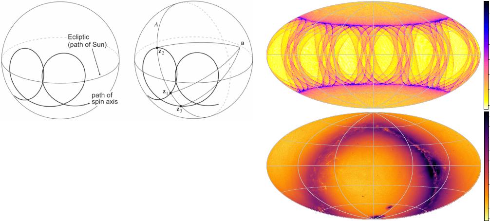
Fig. 1. Overview of the Gaia scanning law. Left: during the nominal
scanning law, the spin axis z makes overlapping loops around the Sun
at a separation of 45
◦
and rate of 5.8 cycles yr
−1
. Right: one source at
point a may be scanned whenever z is 90
◦
from a, that is, on the great
circle A at z
1
, z
2
, z
3
, etc. Reproduction with permission of Fig. 7 in
Gaia Collaboration (2016).
2. How Gaia observes the sky
We start with a brief overview of the Gaia scanning-
law properties that are relevant for this study (for more
details, see Gaia Collaboration 2016; Lindegren & Bastian
2010; de Bruijne et al. 2010). We only consider operations under
the nominal scanning law (NSL) and ignored other non-nominal
modes because they do not affect the majority of the data sig-
nificantly and are not essential for the understanding of the dis-
cussed features. The NSL dictates the way in which the Gaia
spacecraft scans the sky; its two fields of view are separated by
106.5
◦
, and it rotates in a plane orthogonal to the spacecraft spin
axis with a period of 6 h. Each field of view has an instanta-
neous coverage of about 0.5 deg
2
(0.72
◦
× 0.69
◦
), and a source
is typically observed sequentially by at least one pair of the pre-
ceding and following field of view, with decreasing frequency of
longer sequences of recurring observations due to the slow and
non-constant precession rate of the spin axis (see for example
Eyer et al. 2017, for these all-sky sequence statistics). For obser-
vations around a certain time at a specific sky location, a low or
high AC-scan velocity (see Sect. 2.3) will produce more or fewer
sequences of recurring observations, respectively. If the spin axis
had a fixed orientation in space, a single great circle alone would
be scanned on the sky. In reality, the spacecraft orbits the sec-
ond Lagrangian point (L2) of the Earth-Sun system, and thus,
the spacecraft has to rotate its spin axis with a yearly cycle to
keep the instrumentation behind the solar shield. To be able to
acquire useful astrometric measurements throughout the sky (in
terms of temporal sampling and required instrument orientation),
the spin axis is made to precess at a 45
◦
angle around the direc-
tion towards the Sun with a frequency of 5.8 cycles yr
−1
, which
is about 63.0 d per cycle (see the left panel of Fig. 1). To be pre-
cise, this precession is around a fictitious nominal Sun direction
as seen from L2 (that is, along the Earth-Sun vector), and not
from Gaia orbiting L2, although the offset is always less than
0.15
◦
(see Gaia Collaboration 2016). This gives rise to the spe-
cific observation distribution, as illustrated in the top panel of
Fig. 2, along with the published Gaia DR3 source sky density in
the bottom panel for comparison.
Because of the approximately 3:1 aspect ratio of the Gaia
primary mirrors (Gaia Collaboration 2016) and matching 1:3
pixel aspect ratio (to achieve diffraction-limited sampling), the
highest image sampling resolution of 58.9 mas/pixel is achieved
in the so-called along-scan (AL) direction. This is the direction
in which a field of view passes over a particular source due to
20
40
60
80
100
120
140
number of FoV observations
1000
2000
5000
1e4
2e4
5e4
1e5
2e5
5e5
1e6
sources per square degree
Fig. 2. Ecliptic coordinate plots with longitude zero at the centre and
increasing to the left. Top panel: simulated number of field-of-view
observations during the nominal scanning law phase of the Gaia DR3
time range. Bottom panel: sky density of the published Gaia DR3
sources.
the spinning motion of the spacecraft. Its direction is indicated
by the time-dependent scan angle ψ that is illustrated in Fig. 6.
The direction orthogonal to AL is called across-scan (AC), and
it is sampled with a resolution of 176.8 mas/pixel. Depending
on the magnitude of a detected source and the instrument, the
details of the data acquisition vary, as described in Sect. 3.
The most important information in this section is that the
vast majority of Gaia information is encoded and contained in
the AL-scan measurement, which is taken in the direction of the
scan angle over a source at a particular time.
2.1. Scan-angle distribution of source observations
The nominal scanning law not only dictates the cadence and thus
total number of observations for each position on the sky (as
shown in the top panel of Fig. 2), but also the associated obser-
vation scan angles. The scan angle ψ in Fig. 6 at a certain sky
position and time is zero when pointing toward the local equato-
rial north and 90
◦
when pointing towards the local equatorial east
direction. To illustrate the all-sky scan-angle distribution in the
bottom panel of Fig. 3, we collapsed all sky positions along the
ecliptic longitude because the nominal scanning law induces the
most distinctive scan-angle variations as a function of ecliptic
latitude, as also seen in the observation counts of Fig. 3. We use
the hierarchical equal area isolatitude pixelation (HEALPix) of
the celestial sphere (Górski et al. 2002). The normal (equatorial-
based) scan-angle would cause a sky-position-dependent offset
of the scan-angles of a source due to the offset between the
equatorial and ecliptic reference frame, however, thus blurring
the image. To circumvent this issue, we thus introduce the eclip-
tic scan angle, ψ
ecl
, which is defined with respect to the ecliptic
local north and east directions. It effectively is the (equatorial)
scan angle plus an offset that depends on sky position, as given
by Eq. (D.7).
The top panel of Fig. 3 shows the ecliptic scan-angle distri-
bution for sources along a half-circle slice with ecliptic longitude
A25, page 2 of 52
of 52
免费下载
【版权声明】本文为墨天轮用户原创内容,转载时必须标注文档的来源(墨天轮),文档链接,文档作者等基本信息,否则作者和墨天轮有权追究责任。如果您发现墨天轮中有涉嫌抄袭或者侵权的内容,欢迎发送邮件至:contact@modb.pro进行举报,并提供相关证据,一经查实,墨天轮将立刻删除相关内容。
下载排行榜

评论