Machine Learning Super VIP Cheatsheet.pdf

yBmZlQzJ

16页

0次

2024-12-02

免费下载

CS 229 – Machine Learning https://stanford.edu/~shervine

Super VIP Cheatsheet: Machine Learning

Afshine Amidi and Shervine Amidi

September 15, 2018

Contents

1 Supervised Learning 2

1.1 Introduction to Supervised Learning . . . . . . . . . . . . . . . . . . . 2

1.2 Notations and general concepts . . . . . . . . . . . . . . . . . . . . . 2

1.3 Linear models . . . . . . . . . . . . . . . . . . . . . . . . . . . . . . 2

1.3.1 Linear regression . . . . . . . . . . . . . . . . . . . . . . . . . 2

1.3.2 Classiﬁcation and logistic regression . . . . . . . . . . . . . . . 3

1.3.3 Generalized Linear Models . . . . . . . . . . . . . . . . . . . . 3

1.4 Support Vector Machines . . . . . . . . . . . . . . . . . . . . . . . . 3

1.5 Generative Learning . . . . . . . . . . . . . . . . . . . . . . . . . . . 4

1.5.1 Gaussian Discriminant Analysis . . . . . . . . . . . . . . . . . 4

1.5.2 Naive Bayes . . . . . . . . . . . . . . . . . . . . . . . . . . . 4

1.6 Tree-based and ensemble methods . . . . . . . . . . . . . . . . . . . . 4

1.7 Other non-parametric approaches . . . . . . . . . . . . . . . . . . . . 4

1.8 Learning Theory . . . . . . . . . . . . . . . . . . . . . . . . . . . . . 5

2 Unsupervised Learning 6

2.1 Introduction to Unsupervised Learning . . . . . . . . . . . . . . . . . 6

2.2 Clustering . . . . . . . . . . . . . . . . . . . . . . . . . . . . . . . . 6

2.2.1 Expectation-Maximization . . . . . . . . . . . . . . . . . . . . 6

2.2.2 k-means clustering . . . . . . . . . . . . . . . . . . . . . . . . 6

2.2.3 Hierarchical clustering . . . . . . . . . . . . . . . . . . . . . . 6

2.2.4 Clustering assessment metrics . . . . . . . . . . . . . . . . . . 6

2.3 Dimension reduction . . . . . . . . . . . . . . . . . . . . . . . . . . . 7

2.3.1 Principal component analysis . . . . . . . . . . . . . . . . . . 7

2.3.2 Independent component analysis . . . . . . . . . . . . . . . . . 7

3 Deep Learning 8

3.1 Neural Networks . . . . . . . . . . . . . . . . . . . . . . . . . . . . . 8

3.2 Convolutional Neural Networks . . . . . . . . . . . . . . . . . . . . . 8

3.3 Recurrent Neural Networks . . . . . . . . . . . . . . . . . . . . . . . 8

3.4 Reinforcement Learning and Control . . . . . . . . . . . . . . . . . . . 9

4 Machine Learning Tips and Tricks 10

4.1 Metrics . . . . . . . . . . . . . . . . . . . . . . . . . . . . . . . . . . 10

4.1.1 Classiﬁcation . . . . . . . . . . . . . . . . . . . . . . . . . . . 10

4.1.2 Regression . . . . . . . . . . . . . . . . . . . . . . . . . . . . 10

4.2 Model selection . . . . . . . . . . . . . . . . . . . . . . . . . . . . . . 11

4.3 Diagnostics . . . . . . . . . . . . . . . . . . . . . . . . . . . . . . . . 11

5 Refreshers 12

5.1 Probabilities and Statistics . . . . . . . . . . . . . . . . . . . . . . . . 12

5.1.1 Introduction to Probability and Combinatorics . . . . . . . . . 12

5.1.2 Conditional Probability . . . . . . . . . . . . . . . . . . . . . 12

5.1.3 Random Variables . . . . . . . . . . . . . . . . . . . . . . . . 13

5.1.4 Jointly Distributed Random Variables . . . . . . . . . . . . . . 13

5.1.5 Parameter estimation . . . . . . . . . . . . . . . . . . . . . . 14

5.2 Linear Algebra and Calculus . . . . . . . . . . . . . . . . . . . . . . . 14

5.2.1 General notations . . . . . . . . . . . . . . . . . . . . . . . . 14

5.2.2 Matrix operations . . . . . . . . . . . . . . . . . . . . . . . . 15

5.2.3 Matrix properties . . . . . . . . . . . . . . . . . . . . . . . . 15

5.2.4 Matrix calculus . . . . . . . . . . . . . . . . . . . . . . . . . 16

Stanford University 1 Fall 2018

CS 229 – Machine Learning Shervine Amidi & Afshine Amidi

1 Supervised Learning

1.1 Introduction to Supervised Learning

Given a set of data points {x

(1)

, ..., x

(m)

} associated to a set of outcomes {y

(1)

, ..., y

(m)

}, we

want to build a classiﬁer that learns how to predict y from x.

r Type of prediction – The diﬀerent types of predictive models are summed up in the table

below:

Regression Classiﬁer

Outcome Continuous Class

Examples Linear regression Logistic regression, SVM, Naive Bayes

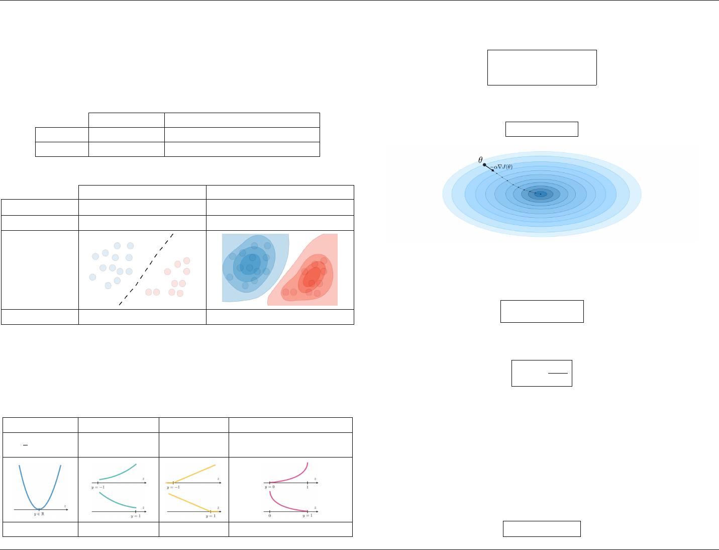
r Type of model – The diﬀerent models are summed up in the table below:

Discriminative model Generative model

Goal Directly estimate P (y|x) Estimate P (x|y) to deduce P (y|x)

What’s learned Decision boundary Probability distributions of the data

Illustration

Examples Regressions, SVMs GDA, Naive Bayes

1.2 Notations and general concepts

r Hypothesis – The hypothesis is noted h

and is the model that we choose. For a given input

data x

(i)

, the model prediction output is h

(i)

r Loss function – A loss function is a function L : (z,y) ∈ R × Y 7−→ L(z,y) ∈ R that takes as

inputs the predicted value z corresponding to the real data value y and outputs how diﬀerent

they are. The common loss functions are summed up in the table below:

Least squared Logistic Hinge Cross-entropy

(y − z)

log(1 + exp(−yz)) max(0,1 − yz) −



y log(z) + (1 − y) log(1 − z)



Linear regression Logistic regression SVM Neural Network

r Cost function – The cost function J is commonly used to assess the performance of a model,

and is deﬁned with the loss function L as follows:

J(θ) =

i=1

L(h

(i)

), y

(i)

)

r Gradient descent – By noting α ∈ R the learning rate, the update rule for gradient descent

is expressed with the learning rate and the cost function J as follows:

θ ←− θ − α∇J (θ)

Remark: Stochastic gradient descent (SGD) is updating the parameter based on each training

example, and batch gradient descent is on a batch of training examples.

r Likelihood – The likelihood of a model L(θ) given parameters θ is used to ﬁnd the optimal

parameters θ through maximizing the likelihood. In practice, we use the log-likelihood `(θ) =

log(L(θ)) which is easier to optimize. We have:

opt

= arg max

L(θ)

r Newton’s algorithm – The Newton’s algorithm is a numerical method that ﬁnds θ such

that `

(θ) = 0. Its update rule is as follows:

θ ← θ −

(θ)

Remark: the multidimensional generalization, also known as the Newton-Raphson method, has

the following update rule:

θ ← θ −



∇

`(θ)



−1

∇

`(θ)

1.3 Linear models

1.3.1 Linear regression

We assume here that y|x; θ ∼ N(µ,σ

)

r Normal equations – By noting X the matrix design, the value of θ that minimizes the cost

function is a closed-form solution such that:

θ = (X

−1

Stanford University 2 Fall 2018

of 16

免费下载

vip

关注

评论