Python气象数据处理与绘图：经验正交分解EOF

1、前言

经验正交函数分析方法(empirical orthogonal function，缩写EOF)也称特征向量分析(eigenvector analysis)，或者主成分分析(principal component analysis)，是一种分析矩阵数据中的结构特征，提取主要数据特征量的一种方法。

2、导入模块

 1import cartopy.crs as ccrs
 2import cartopy.feature as cfeature
 3from netCDF4 import Dataset
 4import matplotlib.pyplot as plt
 5import numpy as np
 6
 7from eofs.standard import Eof
 8from eofs.examples import example_data_path
 9
10import warnings
11warnings.filterwarnings('ignore')

复制

3、冬季北大西洋位势高度数据

北大西洋涛动（North Atlantic oscillation，NAO）于1920年由Sir Gilbert Walker（G.沃克）发现，三大涛动之一，指亚速尔高压和冰岛低压之间气压的反向变化关系，即当亚速尔地区气压偏高时，冰岛地区气压偏低，反之亦然。NAO是北大西洋地区大气最显著的模态。其气候影响最突出的主要是北美及欧洲,但也可能对其它地区如亚洲的气候有一定影响。

 1# Read geopotential height data using the netCDF4 module. The file contains
 2# December-February averages of geopotential height at 500 hPa for the
 3# European/Atlantic domain (80W-40E, 20-90N).
 4filename = '../input/eof7091/hgt_djf.nc'
 5ncin = Dataset(filename, 'r')
 6z_djf = ncin.variables['z'][:]
 7lons = ncin.variables['longitude'][:]
 8lats = ncin.variables['latitude'][:]
 9ncin.close()
10
11# Compute anomalies by removing the time-mean.
12z_djf_mean = z_djf.mean(axis=0)
13z_djf = z_djf - z_djf_mean
14
15# Create an EOF solver to do the EOF analysis. Square-root of cosine of
16# latitude weights are applied before the computation of EOFs.
17coslat = np.cos(np.deg2rad(lats)).clip(0., 1.)
18wgts = np.sqrt(coslat)[..., np.newaxis]
19solver = Eof(z_djf, weights=wgts)
20
21# Retrieve the leading EOF, expressed as the covariance between the leading PC
22# time series and the input SLP anomalies at each grid point.
23eof1 = solver.eofsAsCovariance(neofs=1)
24
25# Plot the leading EOF expressed as covariance in the European/Atlantic domain.
26clevs = np.linspace(-75, 75, 11)
27proj = ccrs.Orthographic(central_longitude=-20, central_latitude=60)
28ax = plt.axes(projection=proj)
29ax.set_global()
30ax.coastlines()
31ax.contourf(lons, lats, eof1.squeeze(), levels=clevs,
32            cmap=plt.cm.RdBu_r, transform=ccrs.PlateCarree())
33plt.title('EOF1 expressed as covariance', fontsize=16)
34
35plt.show()

复制

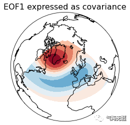
北大西洋上两个大气活动中心（冰岛低压和亚速尔高压）的气压变化为明显负相关；当冰岛低压加深时，亚速尔高压加强，或冰岛低压填塞时，亚速尔高压减弱。G.沃克称这一现象为北大西洋涛动North Atlantic oscillation (NAO)。北大西洋涛动强，表明两个活动中心之间的气压差大，北大西洋中纬度的西风强，为高指数环流。这时墨西哥湾暖流及拉布拉多寒流均增强，西北欧和美国东南部因受强暖洋流影响，出现暖冬；同时为寒流控制的加拿大东岸及格陵兰西岸却非常寒冷。反之北大西洋涛动弱，表明两个活动中心之间的气压差小，北大西洋上西风减弱，为低指数环流。这时西北欧及美国东南部将出现冷冬，而加拿大东岸及格陵兰西岸则相对温暖。

4、太平洋海温距平数据

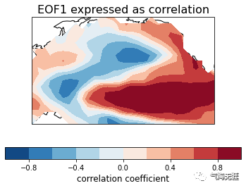
厄尔尼诺现象，是指东太平洋海水每隔数年就会异常升温的现象，是厄尔尼诺-南方振荡现象（El Niño-Southern Oscillation，ENSO）中，东太平洋升温的阶段。它与中太平洋和东太平洋（约在国际换日线及西经120度）赤道位置产生的温暖海流有关。厄尔尼诺-南方振荡现象是指中太平洋和东太平洋赤道位置海面温度的高低温循环。厄尔尼诺现象是因为西太平洋的高气压及东太平洋的低气压所造成。厄尔尼诺-南方振荡现象中的低温阶段称为拉尼娜现象（也称为反圣婴现象），是指东太平洋的海面温度高于平均值，以及西太平洋的气压较低及东太平洋的气压较高所造成。

 1"""
 2Compute and plot the leading EOF of sea surface temperature in the
 3central and northern Pacific during winter time.
 4
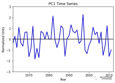
 5The spatial pattern of this EOF is the canonical El Nino pattern, and
 6the associated time series shows large peaks and troughs for well-known
 7El Nino and La Nina events.
 8"""
 9filename = '../input/eof7091/sst_ndjfm_anom.nc'
10ncin = Dataset(filename, 'r')
11sst = ncin.variables['sst'][:]
12lons = ncin.variables['longitude'][:]
13lats = ncin.variables['latitude'][:]
14ncin.close()
15
16# Create an EOF solver to do the EOF analysis. Square-root of cosine of
17# latitude weights are applied before the computation of EOFs.
18coslat = np.cos(np.deg2rad(lats))
19wgts = np.sqrt(coslat)[..., np.newaxis]
20solver = Eof(sst, weights=wgts)
21
22# Retrieve the leading EOF, expressed as the correlation between the leading
23# PC time series and the input SST anomalies at each grid point, and the
24# leading PC time series itself.
25eof1 = solver.eofsAsCorrelation(neofs=1)
26pc1 = solver.pcs(npcs=1, pcscaling=1)
27
28# Plot the leading EOF expressed as correlation in the Pacific domain.
29clevs = np.linspace(-1, 1, 11)
30ax = plt.axes(projection=ccrs.PlateCarree(central_longitude=190))
31fill = ax.contourf(lons, lats, eof1.squeeze(), clevs,
32                   transform=ccrs.PlateCarree(), cmap=plt.cm.RdBu_r)
33ax.add_feature(cfeature.LAND, facecolor='w', edgecolor='k')
34cb = plt.colorbar(fill, orientation='horizontal')
35cb.set_label('correlation coefficient', fontsize=12)
36plt.title('EOF1 expressed as correlation', fontsize=16)
37
38# Plot the leading PC time series.
39plt.figure()
40years = range(1962, 2012)
41plt.plot(years, pc1, color='b', linewidth=2)
42plt.axhline(0, color='k')
43plt.title('PC1 Time Series')
44plt.xlabel('Year')
45plt.ylabel('Normalized Units')
46plt.xlim(1962, 2012)
47plt.ylim(-3, 3)
48plt.show()

复制